Topic Model API and Usage

Topic models are useful, but the R ecosystem exposes them through several different object types, argument names, and output formats. That makes it harder than it should be to compare models, reuse diagnostics, or move a workflow from one backend to another.

NLPstudio’s topic-model API is built to remove that friction. The package gives you one workflow for fitting, inspecting, predicting, evaluating, selecting, and summarizing topic models. The backend can change, but the main verbs and the standardized outputs stay the same.

This vignette walks through that workflow from start to finish. We will prepare a small corpus, fit one topic model, inspect the standardized outputs, evaluate the model, compare candidate values of k, assess seed stability, build an interpretation table, and sketch how the same calls transfer to other engines.

The notation follows Lewis and Grossetti (2022). In particular, this vignette uses DTW for document-topic weights and TWW for topic-word weights. Those two tables are the main package-standard representation of a fitted topic model: DTW describes documents in the topic space, while TWW describes topics in the vocabulary space.

The package currently supports topic models from text2vec, topicmodels, seededlda, optionally stm, and optionally topicmodels.etm. To keep this vignette fast and reliable during package checks, only the topicmodels examples are evaluated. The other backend sections are included as non-evaluated templates so you can see the same API shape without requiring every optional backend on your machine.

Public API Stability

NLPstudio v1.0.0 freezes the core topic-model output shapes as public contracts. An nlp_topic_fit stores the standardized model pieces, evaluate_topic_model() and select_k_topics() return long tables with stable metric columns, assess_topic_stability() returns matched-topic stability rows, and the topic summary helpers return one row per topic.

One practical consequence is that evaluation and selection tables retain the same standard columns even when a result is aggregate-only. The columns metric, level, topic_id, value, and supported stay present; aggregate rows use topic_id = NA rather than dropping the column. This makes joins, plots, exports, and downstream summaries predictable.

New code should also use only the final metric names. For example, request held_out_perplexity explicitly rather than the removed "perplexity" alias.

Prepare Data Once

The workflow starts with ordinary data: one row per document, one text column, and any metadata that helps interpret the documents later. Here the metadata is minimal, but the same pattern works with richer document-level fields such as firm identifiers, filing dates, industries, countries, or human-coded labels.

Topic models are estimated from a document-feature matrix. The metadata does not enter the model directly in this example, but we keep it next to the model so it can be returned by downstream helpers. That is what lets later calls attach text, groups, and document identifiers to predictions, representative documents, and summary tables.

library(NLPstudio)
#> ── NLPstudio 1.0.1 ────────────────── https://github.com/contefranz/NLPstudio ──
#> Core imports: cli, data.table, ggplot2, Matrix, methods, quanteda,
#>               quanteda.textstats
#> Optional backends: text2vec, topicmodels, seededlda, stm,
#>                    topicmodels.etm, torch, spacyr, tidytext,
#>                    RcppSimdJson, uwot
#> Use library(<pkg>) to attach any of these to your session.
#> Optional packages are only needed for the functions that use them.
library(quanteda)
#> Package version: 4.4
#> Unicode version: 15.1
#> ICU version: 74.2
#> Parallel computing: disabled
#> See https://quanteda.io for tutorials and examples.

docs <- data.frame(
  doc_id = paste0("doc", 1:10),
  text = c(
    "Revenue growth improved after subscription demand increased.",
    "Recurring software revenue supported customer retention.",
    "Cloud infrastructure costs declined and operating margin expanded.",
    "Capital allocation reflected debt covenants and interest expense.",
    "Audit committee oversight focused on internal control remediation.",
    "Risk disclosures emphasized liquidity and refinancing pressure.",
    "Cybersecurity controls shaped technology governance disclosures.",
    "Management discussed compliance monitoring and reporting quality.",
    "Subscription renewals improved annual recurring revenue trends.",
    "Debt refinancing reduced interest expense and liquidity risk."
  ),
  group = rep(c("performance", "governance"), each = 5),
  stringsAsFactors = FALSE
)

corp <- quanteda::corpus(docs, text_field = "text", docid_field = "doc_id")
toks <- quanteda::tokens(corp, remove_punct = TRUE)
toks <- quanteda::tokens_tolower(toks)
toks <- quanteda::tokens_remove(toks, pattern = quanteda::stopwords("en"))
dfm <- quanteda::dfm(toks)
dfm
#> Document-feature matrix of: 10 documents, 53 features (87.74% sparse) and 1 docvar.
#>       features
#> docs   revenue growth improved subscription demand increased recurring software
#>   doc1       1      1        1            1      1         1         0        0
#>   doc2       1      0        0            0      0         0         1        1
#>   doc3       0      0        0            0      0         0         0        0
#>   doc4       0      0        0            0      0         0         0        0
#>   doc5       0      0        0            0      0         0         0        0
#>   doc6       0      0        0            0      0         0         0        0
#>       features
#> docs   supported customer
#>   doc1         0        0
#>   doc2         1        1
#>   doc3         0        0
#>   doc4         0        0
#>   doc5         0        0
#>   doc6         0        0
#> [ reached max_ndoc ... 4 more documents, reached max_nfeat ... 43 more features ]

Fit One Model

fit_topic_model() is the basic modeling verb. One call means one model specification: one input matrix, one engine, one model family, one value of k, and one set of backend controls.

The object returned by fit_topic_model() is an nlp_topic_fit. It keeps the original backend model, but it also stores the package-owned pieces that make the rest of the API consistent: document-topic weights (DTW), topic-word weights (TWW), stable topic identifiers, the fitted vocabulary, optional document metadata, backend controls, and available hyperparameters.

fit <- fit_topic_model(
  dfm,
  engine = "topicmodels",
  model = "lda",
  method = "Gibbs",
  k = 2,
  doc_data = docs,
  control = list(fit = list(seed = 1L, iter = 75L, burnin = 0L, thin = 1L))
)

fit
#> <nlp_topic_fit>
#>   engine: topicmodels
#>   model: lda (Gibbs)
#>   documents: 10
#>   topics: 2
#>   terms: 53
#>   cached DTW: TRUE
#>   cached TWW: TRUE
#>   stored docvars: TRUE
#>   stored doc_data: TRUE

The printed object is intentionally compact. It tells you what was fit and gives you enough context to confirm that the model has the expected engine, model family, topic count, document count, and vocabulary size.

Notice the topic labels. Standardized outputs use identifiers such as Topic001 and Topic002. Those labels are generated by NLPstudio rather than by a specific backend, which is what allows the same helper functions to work across engines.

Inspect Standardized Outputs

After fitting, the first question is usually: “What did the model learn?” NLPstudio answers that with two standardized tables.

Use get_dtw() for document-topic weights. Each row corresponds to a document, and the Topic### columns describe how much of that document is associated with each topic. Use get_tww() for topic-word weights. Each row corresponds to a topic, and the columns describe the topic’s distribution over the fitted vocabulary.

dtw <- get_dtw(fit, docvars = TRUE, include_text = TRUE)
tww <- get_tww(fit)

head(dtw)
#>    doc_id       group  Topic001  Topic002 topic_max_id topic_max_int
#>    <char>      <char>     <num>     <num>       <char>         <int>
#> 1:   doc1 performance 0.4642857 0.5357143     Topic002             2
#> 2:   doc2 performance 0.5000000 0.5000000     Topic001             1
#> 3:   doc3 performance 0.4561404 0.5438596     Topic002             2
#> 4:   doc4 performance 0.5614035 0.4385965     Topic001             1
#> 5:   doc5 performance 0.4912281 0.5087719     Topic002             2
#> 6:   doc6  governance 0.5000000 0.5000000     Topic001             1
#>    topic_max_value
#>              <num>
#> 1:       0.5357143
#> 2:       0.5000000
#> 3:       0.5438596
#> 4:       0.5614035
#> 5:       0.5087719
#> 6:       0.5000000
#>                                                                  text
#>                                                                <char>
#> 1:       Revenue growth improved after subscription demand increased.
#> 2:           Recurring software revenue supported customer retention.
#> 3: Cloud infrastructure costs declined and operating margin expanded.
#> 4:  Capital allocation reflected debt covenants and interest expense.
#> 5: Audit committee oversight focused on internal control remediation.
#> 6:    Risk disclosures emphasized liquidity and refinancing pressure.
tww[, 1:6, with = FALSE]
#>    topic_id     revenue      growth    improved subscription      demand
#>      <char>       <num>       <num>       <num>        <num>       <num>
#> 1: Topic001 0.002680965 0.002680965 0.002680965  0.002680965 0.029490617
#> 2: Topic002 0.080939948 0.028720627 0.054830287  0.054830287 0.002610966

The full TWW matrix is useful for computation, but it is often too wide for human reading. When the goal is interpretation, get_top_terms() returns the most important words for each topic in either long or wide format. It accepts a fitted model or a TWW table, so you can use it early in exploration or later in a reporting pipeline.

top_terms <- get_top_terms(fit, n = 5, format = "long")
top_terms
#>      rank    topic         term probability
#>     <int>   <char>       <char>       <num>
#>  1:     1 Topic001         debt  0.05630027
#>  2:     2 Topic001     interest  0.05630027
#>  3:     3 Topic001      expense  0.05630027
#>  4:     4 Topic001         risk  0.05630027
#>  5:     5 Topic001    liquidity  0.05630027
#>  6:     1 Topic002      revenue  0.08093995
#>  7:     2 Topic002     improved  0.05483029
#>  8:     3 Topic002 subscription  0.05483029
#>  9:     4 Topic002    recurring  0.05483029
#> 10:     5 Topic002  disclosures  0.05483029

get_top_terms(tww, n = 3, format = "wide")
#>     rank Topic001_term Topic001_prob Topic002_term Topic002_prob
#>    <int>        <char>         <num>        <char>         <num>
#> 1:     1          debt    0.05630027       revenue    0.08093995
#> 2:     2      interest    0.05630027      improved    0.05483029
#> 3:     3       expense    0.05630027  subscription    0.05483029

Some engines expose topic-model hyperparameters, while others expose only part of that information. NLPstudio returns what is available through get_topic_hyperparameters() in a backend-neutral table. The original backend controls are still stored on fit$backend_control, which is helpful when you need to audit exactly how a model was estimated.

get_topic_hyperparameters(fit)
#>    parameter  value source_section source_name
#>       <char> <AsIs>         <char>      <char>
#> 1:         k      2       argument           k
#> 2:     alpha     25   model_object       alpha
#> 3:      beta    0.1            fit       delta

Interpret Topics

Topic interpretation usually combines two views. The first is lexical: which words define the topic? The second is documentary: which documents are strongest examples of the topic?

For the lexical view, plot_top_terms() uses the long output from get_top_terms(). The plot is a quick check on whether the discovered topics look distinct and interpretable.

plot_top_terms(top_terms)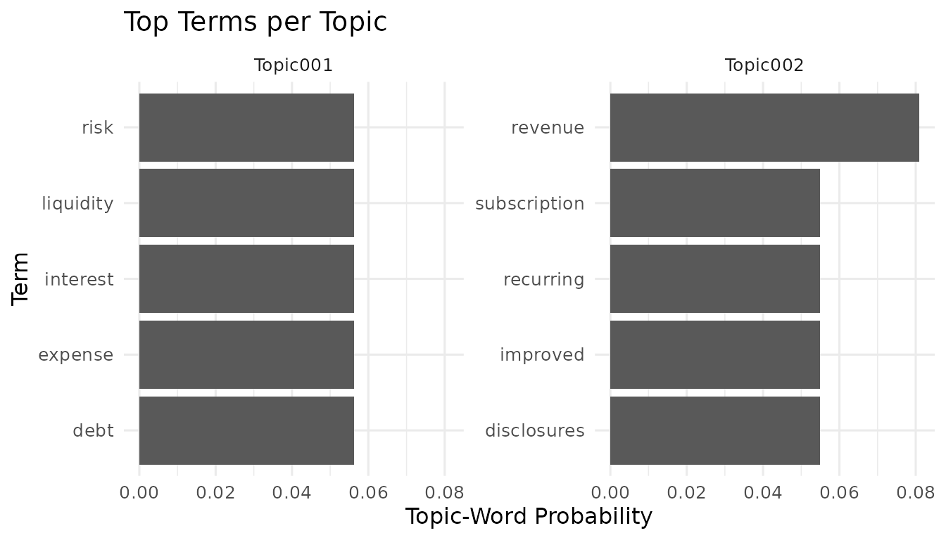

plot_dtw() gives the document-side view. It shows how topic weights are spread across documents, which helps you see whether the fitted topics dominate a few documents, appear broadly across the corpus, or remain very diffuse.

plot_dtw(fit)
#> `stat_bin()` using `bins = 30`. Pick better value `binwidth`.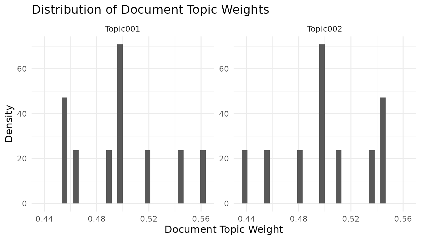

Representative documents are often the easiest way to name and validate a topic. get_representative_candidates() ranks documents by their dominant topic weight and assigns simple candidate bands. If metadata or text are available, the function can return them with the ranking so you can inspect the examples in context.

representatives <- get_representative_candidates(
  fit,
  doc_data = docs,
  include_text = TRUE
)

representatives[
  ,
  .(doc_id, topic_max_id, topic_max_value, candidate_band, topic_rank, text)
]
#>     doc_id topic_max_id topic_max_value candidate_band topic_rank
#>     <char>       <char>           <num>         <char>      <int>
#>  1:   doc4     Topic001       0.5614035          VHIGH          1
#>  2:  doc10     Topic001       0.5438596           HIGH          2
#>  3:   doc8     Topic001       0.5178571           HIGH          3
#>  4:   doc2     Topic001       0.5000000           VLOW          4
#>  5:   doc6     Topic001       0.5000000           VLOW          5
#>  6:   doc7     Topic001       0.5000000            LOW          6
#>  7:   doc3     Topic002       0.5438596           HIGH          1
#>  8:   doc9     Topic002       0.5438596          VHIGH          2
#>  9:   doc1     Topic002       0.5357143            LOW          3
#> 10:   doc5     Topic002       0.5087719           VLOW          4
#>                                                                   text
#>                                                                 <char>
#>  1:  Capital allocation reflected debt covenants and interest expense.
#>  2:      Debt refinancing reduced interest expense and liquidity risk.
#>  3:  Management discussed compliance monitoring and reporting quality.
#>  4:           Recurring software revenue supported customer retention.
#>  5:    Risk disclosures emphasized liquidity and refinancing pressure.
#>  6:   Cybersecurity controls shaped technology governance disclosures.
#>  7: Cloud infrastructure costs declined and operating margin expanded.
#>  8:    Subscription renewals improved annual recurring revenue trends.
#>  9:       Revenue growth improved after subscription demand increased.
#> 10: Audit committee oversight focused on internal control remediation.

Predict New Documents

Once a model is fit, you may want to score new documents against the same topic space. predict_topic_model() handles the practical detail that new documents rarely have exactly the same vocabulary columns as the training matrix. The new input is aligned to the fitted vocabulary before backend prediction, and the returned DTW table uses the same Topic### naming contract as the fitted model.

new_docs <- data.frame(
  doc_id = paste0("new", 1:3),
  text = c(
    "Recurring revenue improved after subscription renewals.",
    "Audit remediation and compliance controls remained a priority.",
    "Debt refinancing lowered liquidity risk and interest expense."
  ),
  source = c("forecast", "governance", "capital"),
  stringsAsFactors = FALSE
)

new_corp <- quanteda::corpus(new_docs, text_field = "text", docid_field = "doc_id")
new_toks <- quanteda::tokens(new_corp, remove_punct = TRUE)
new_toks <- quanteda::tokens_tolower(new_toks)
new_toks <- quanteda::tokens_remove(new_toks, pattern = quanteda::stopwords("en"))
new_dfm <- quanteda::dfm(new_toks)

pred <- predict_topic_model(
  fit,
  new_dfm,
  doc_data = new_docs,
  include_text = TRUE
)
#> Warning: Dropping 3 terms that were not found in the fitted vocabulary.

pred
#>    doc_id     source  Topic001  Topic002 topic_max_id topic_max_int
#>    <char>     <char>     <num>     <num>       <char>         <int>
#> 1:   new1   forecast 0.4545455 0.5454545     Topic002             2
#> 2:   new2 governance 0.5000000 0.5000000     Topic001             1
#> 3:   new3    capital 0.5357143 0.4642857     Topic001             1
#>    topic_max_value
#>              <num>
#> 1:       0.5454545
#> 2:       0.5000000
#> 3:       0.5357143
#>                                                              text
#>                                                            <char>
#> 1:        Recurring revenue improved after subscription renewals.
#> 2: Audit remediation and compliance controls remained a priority.
#> 3:  Debt refinancing lowered liquidity risk and interest expense.

Evaluate Model Quality

Interpretability is not only visual. evaluate_topic_model() collects common quality metrics into one long-format table so they can be compared, plotted, or joined to model-selection results. Some metrics summarize the whole model; others are defined topic by topic. Setting level = "all" returns both where available.

evaluation <- evaluate_topic_model(
  fit,
  training = dfm,
  metrics = c("coherence_umass", "diversity", "exclusivity", "train_perplexity"),
  top_n = 5L,
  level = "all"
)

evaluation
#>              metric     level topic_id       value supported
#>              <char>    <char>   <char>       <num>    <lgcl>
#> 1:  coherence_umass aggregate     <NA>  -6.0231856      TRUE
#> 2:  coherence_umass     topic Topic001  -0.4158883      TRUE
#> 3:  coherence_umass     topic Topic002 -11.6304828      TRUE
#> 4:        diversity aggregate     <NA>   1.0000000      TRUE
#> 5:      exclusivity aggregate     <NA>   0.9559872      TRUE
#> 6:      exclusivity     topic Topic001   0.9556797      TRUE
#> 7:      exclusivity     topic Topic002   0.9562947      TRUE
#> 8: train_perplexity aggregate     <NA>  48.3734452      TRUE

Select K

Choosing the number of topics is a modeling decision, not just a software argument. select_k_topics() makes that decision easier to inspect by fitting a grid of candidate topic counts and returning the requested metrics in one selection table.

The default behavior remains the simple path: fit each value of k once and evaluate it. When stability_seeds is supplied, each candidate k is also refit across those seeds. The selection table then includes aggregate stability, and the full stability details are attached as an attribute for deeper inspection.

k_selection <- select_k_topics(
  dfm,
  engine = "topicmodels",
  model = "lda",
  method = "Gibbs",
  k_grid = 2:3,
  metrics = c("coherence_umass", "diversity", "exclusivity"),
  top_n = 5L,
  holdout = 0,
  seed = 10L,
  stability_seeds = c(1L, 2L),
  control = list(fit = list(iter = 75L, burnin = 0L, thin = 1L))
)

k_selection
#> <nlp_k_selection>
#>   K grid:  2, 3
#>   metrics: coherence_umass, diversity, exclusivity, stability
#> 
#>   stability: included
#> 
#>   Best K per metric (aggregate level):
#>     coherence_umass      K = 3  (-17.21)
#>     diversity            K = 2  (1) [tied]
#>     exclusivity          K = 2  (0.9523)
#>     stability            K = 2  (0.6858)
attr(k_selection, "stability")$k2
#> <nlp_topic_stability>
#>   K: 2
#>   runs compared: 1
#>   aggregate stability: 0.6858

For reporting, the long selection table is often too detailed. A paper or appendix usually needs one row per candidate k, with the aggregate evidence side by side. summarize_k_selection() creates that table and preserves topic-level rows as an attribute when they are present.

k_report <- summarize_k_selection(k_selection)
k_report
#> <nlp_k_selection_summary>
#>   candidate K values: 2, 3
#>   columns: coherence_umass, diversity, exclusivity, stability
#>   OpTop: not included

Assess Stability Directly

Topic models can move when the random seed changes. That does not necessarily mean a model is bad, but it is information you should see before treating topic labels as stable research objects.

assess_topic_stability() makes that check explicit. In the automatic workflow, it repeatedly calls fit_topic_model() with the same model specification and different seeds. Unless you supply resampling, the seed is the only thing that changes across runs.

Topic labels are arbitrary across repeated runs. A topic called Topic001 in one seed may correspond to Topic002 in another seed. The stability helper therefore extracts standardized TWW from each run, aligns vocabularies, matches topics across runs, and reports matched-topic cosine similarities.

stability <- assess_topic_stability(
  dfm,
  engine = "topicmodels",
  model = "lda",
  method = "Gibbs",
  k = 2,
  seeds = 1:3,
  control = list(fit = list(iter = 75L, burnin = 0L, thin = 1L))
)

stability
#> <nlp_topic_stability>
#>   K: 2
#>   runs compared: 2
#>   aggregate stability: 0.6385

If you prefer to fit models yourself, you can still use the same matching and scoring code. Pass a list of nlp_topic_fit objects, and assess_topic_stability() will skip fitting and move directly to standardized TWW extraction, topic matching, and stability scoring.

fits <- lapply(1:3, function(seed) {
  fit_topic_model(
    dfm,
    engine = "topicmodels",
    model = "lda",
    method = "Gibbs",
    k = 2,
    control = list(fit = list(seed = seed, iter = 75L, burnin = 0L, thin = 1L))
  )
})

assess_topic_stability(fits, seeds = 1:3)
#> <nlp_topic_stability>
#>   K: 2
#>   runs compared: 2
#>   aggregate stability: 0.6385

Summarize and Export

After fitting, inspecting, evaluating, and checking stability, the next step is usually a table that can be reviewed, exported, or adapted for a paper appendix. summarize_topics() builds that table directly from the fitted object. It returns one row per topic with top terms, top-term probabilities, topic prevalence, available metrics, representative documents, and optional text or metadata.

topic_summary <- summarize_topics(
  fit,
  training = dfm,
  doc_data = docs,
  top_n = 5L,
  representative_n = 2L,
  include_text = TRUE
)

topic_summary
#>    topic_id topic_int                                               top_terms
#>      <char>     <int>                                                  <char>
#> 1: Topic001         1                debt, interest, expense, risk, liquidity
#> 2: Topic002         2 revenue, improved, subscription, recurring, disclosures
#>                                   top_term_probabilities prevalence
#>                                                   <char>      <num>
#> 1: 0.0563003, 0.0563003, 0.0563003, 0.0563003, 0.0563003  0.4990915
#> 2: 0.0809399, 0.0548303, 0.0548303, 0.0548303, 0.0548303  0.5009085
#>    coherence_npmi coherence_umass diversity exclusivity representative_doc_ids
#>             <num>           <num>     <num>       <num>                 <char>
#> 1:     0.63876401      -0.4158883         1   0.9556797            doc4, doc10
#> 2:     0.04913968     -11.6304828         1   0.9562947             doc3, doc9
#>    representative_documents
#>                      <list>
#> 1:        <data.table[2x2]>
#> 2:        <data.table[2x2]>
#>                                                                                                                      representative_text
#>                                                                                                                                   <char>
#> 1:    Capital allocation reflected debt covenants and interest expense. || Debt refinancing reduced interest expense and liquidity risk.
#> 2: Cloud infrastructure costs declined and operating margin expanded. || Subscription renewals improved annual recurring revenue trends.

The summary includes a representative_documents list column. That is useful inside R because each topic can carry its own small document table. For flat file exports, drop the list column and write the remaining scalar columns.

export_summary <- data.table::copy(topic_summary)
export_summary[, representative_documents := NULL]
data.table::fwrite(export_summary, tempfile(fileext = ".csv"))

Adopt Existing Topic Models

You do not have to refit a model just to use the current API. Many projects already have topic models saved from earlier analyses, from direct backend calls, or from older NLPstudio workflows. as_nlp_topic_fit() is the adoption path for those objects. It wraps the existing fit, standardizes the cached DTW and TWW matrices where available, and keeps the original backend object as model_object.

The conversion is deliberately non-refitting. For topicmodels fits, the adapter reads the fitted gamma, beta, terms, document IDs, controls, and hyperparameters from the S4 object. For seededlda, it uses the stored theta, phi, k, alpha, and beta. For raw text2vec WarpLDA/LDA objects, the topic-word distribution can be recovered from the model object, but the document-topic matrix is not stored by text2vec itself; pass the theta matrix returned by fit_transform() when you need DTW access.

# topicmodels::LDA() or topicmodels::CTM()
topicmodels_fit <- as_nlp_topic_fit(existing_topicmodels_fit)

# seededlda::textmodel_lda() or seededlda::textmodel_seededlda()
seededlda_fit <- as_nlp_topic_fit(existing_seededlda_fit)

# raw text2vec::LDA() / WarpLDA object
text2vec_fit <- as_nlp_topic_fit(raw_text2vec_fit, theta = saved_theta)

# sequential LDA from seededlda is not reliably distinguishable after fitting
seqlda_fit <- as_nlp_topic_fit(existing_seededlda_fit, model = "seqlda")

# stm::stm() without content covariates
stm_fit <- as_nlp_topic_fit(existing_stm_fit, doc_ids = existing_doc_ids)

Older NLPstudio projects may also contain saved outputs from the removed warp_lda() wrapper. Those list objects usually contain lda_object, theta, and phi. The adapter uses theta as DTW, phi as TWW, and keeps the original WarpLDA backend object.

old <- readRDS("legacy-warp-lda-output.rds")
legacy_fit <- as_nlp_topic_fit(old)

get_dtw(legacy_fit)
get_tww(legacy_fit)
get_top_terms(legacy_fit, n = 10)
summarize_topics(legacy_fit, training = original_dfm)

If an adopted object is missing DTW or TWW, the adapter preserves the parts that are available and warns about the missing cache. Functions that need the missing component will then fail with the same messages used by current partial nlp_topic_fit objects.

Use OpTop with NLPstudio Fits

Some research workflows use the OpTop package to select the number of topics with the chi-square testing approach of Lewis and Grossetti (2022). NLPstudio does not reimplement that test. Instead, it prepares the exact objects that OpTop::optimal_topic() expects: an ordered list of raw topicmodels LDA VEM fits and a DFM weighted to document-level word proportions.

This bridge is intentionally narrow. Current OpTop expects LDA_VEM objects from topicmodels::LDA(), so as_optop_input() rejects Gibbs LDA, CTM, text2vec, seededlda, and ETM fits. That strictness is useful: it keeps the statistical test tied to the model class for which OpTop was written.

selection <- select_k_topics(
  dfm,
  engine = "topicmodels",
  model = "lda",
  method = "VEM",
  k_grid = 2:5,
  metrics = c("diversity", "exclusivity"),
  holdout = 0,
  return_fits = TRUE,
  control = list(fit = list(seed = 1))
)

optop_input <- as_optop_input(
  selection,
  weighted_dfm = as_optop_weighted_dfm(dfm)
)

OpTop::optimal_topic(
  lda_models = optop_input$lda_models,
  weighted_dfm = optop_input$weighted_dfm,
  q = 0.8,
  alpha = 0.05,
  do_plot = FALSE
)

If you run OpTop externally, pass the returned table back to summarize_k_selection() to build one export-ready selection report. NLPstudio parses the common OpTop output columns topic, OpTop, and pval, then merges them by k.

optop_result <- OpTop::optimal_topic(
  lda_models = optop_input$lda_models,
  weighted_dfm = optop_input$weighted_dfm,
  q = 0.8,
  alpha = 0.05,
  do_plot = FALSE
)

k_report <- summarize_k_selection(selection, optop = optop_result)
data.table::fwrite(k_report, tempfile(fileext = ".csv"))

Backend Portability

The point of the API is that the workflow above does not belong only to one backend. The fitting controls differ by engine, but the surrounding calls stay recognizable: fit a model, extract DTW/TWW, interpret top terms, evaluate, and summarize.

The examples below are not evaluated in this vignette because optional backend availability varies across machines and CI environments. They are meant as templates for moving the same workflow to another estimator.

fit_text2vec <- fit_topic_model(
  dfm,
  engine = "text2vec",
  model = "lda",
  k = 2,
  control = list(fit = list(n_iter = 100, progressbar = FALSE))
)

get_top_terms(fit_text2vec, n = 5)
evaluate_topic_model(fit_text2vec, training = dfm, metrics = c("diversity", "exclusivity"))

fit_seededlda <- fit_topic_model(
  dfm,
  engine = "seededlda",
  model = "lda",
  k = 2
)

get_dtw(fit_seededlda)
get_tww(fit_seededlda)

Seeded LDA uses the same wrapper but requires a dictionary. Once the model is fit, the downstream accessors remain the same.

seed_dict <- quanteda::dictionary(list(
  performance = c("revenue", "subscription", "margin"),
  governance = c("audit", "control", "compliance")
))

fit_seeded <- fit_topic_model(
  dfm,
  engine = "seededlda",
  model = "seededlda",
  dictionary = seed_dict
)

summarize_topics(fit_seeded, doc_data = docs)

Structural Topic Models: Prevalence and Interpretation

Structural topic models are available through the optional stm backend. In NLPstudio, STM is treated as an extension of the same topic-model API rather than as a separate workflow. That means the fitted object still has standardized DTW and TWW outputs, stable Topic### identifiers, generic top-term accessors, and the same topic-summary surface used by the other backends.

The important difference is the role of document metadata. With ordinary LDA fits, metadata can be attached after fitting so tables are easier to read. With STM prevalence models, metadata enters the model itself: the prevalence formula describes how document-level variables are associated with topic proportions. That association is estimated by the STM backend and is later reported by estimate_stm_topic_effects().

The example below uses a document variable named group. The call keeps docvars = TRUE so NLPstudio stores the fitted document metadata and can reuse it when estimating topic effects. Users can instead pass explicit metadata to control$fit$data at fitting time, and to estimate_stm_topic_effects() when reporting effects.

library(stm)

dfm_stm <- dfm
quanteda::docvars(dfm_stm, "group") <- docs$group

fit_stm <- fit_topic_model(
  dfm_stm,
  engine = "stm",
  model = "stm",
  k = 2,
  docvars = TRUE,
  control = list(
    fit = list(
      prevalence = ~ group,
      seed = 1L,
      max.em.its = 25L,
      init.type = "Spectral",
      verbose = FALSE
    )
  )
)

Once the model is fit, start with the same standardized outputs used elsewhere in this vignette. get_dtw() gives document-topic weights and can include stored docvars. get_top_terms() reports probability-ranked terms from the standardized TWW matrix. summarize_topics() remains the backend-agnostic interpretation table.

get_dtw(fit_stm, docvars = TRUE)
get_top_terms(fit_stm, n = 5)
summarize_topics(fit_stm, training = dfm_stm, doc_data = docs)

STM also has label families that are useful for interpretation but are not the same object as the standardized TWW matrix. get_stm_topic_labels() exposes those STM-native labels in long format. Probability labels are useful for checking the highest-probability words. FREX, lift, and score labels emphasize different balances between frequency and distinctiveness. NLPstudio does not replace one with another; it returns the label family explicitly so the choice is visible in downstream tables.

summarize_stm_topics() is the report-oriented version. It starts from summarize_topics() and adds collapsed STM label columns so each Topic### row can be reviewed alongside prevalence, generic metrics, and representative documents.

get_stm_topic_labels(
  fit_stm,
  n = 5,
  label_types = c("prob", "frex", "lift", "score")
)

summarize_stm_topics(fit_stm, training = dfm_stm, doc_data = docs)

For prevalence models, the natural final question is not only “what are the topics?” but also “how do document variables relate to topic prevalence?” estimate_stm_topic_effects() answers that question by calling the STM backend and returning coefficient rows in a tidy table. The estimates should be read as model-based associations under the fitted STM specification and the user’s covariate coding. NLPstudio keeps the raw STM effect object attached as an attribute for users who need backend-native follow-up analysis, but the main return value is designed for tables and reproducible reporting.

stm_effects <- estimate_stm_topic_effects(
  fit_stm,
  topics = c("Topic001", "Topic002"),
  nsims = 25
)

stm_effects

This STM support is intentionally bounded. STM prevalence covariates are supported because each topic still has one topic-word distribution and the standardized TWW contract remains valid. STM content covariates are not supported: they allow word distributions to vary by covariate level, which means a single ordinary TWW row per topic would hide part of the fitted model. Prediction for STM prevalence fits is also not inferred automatically, because new-document prediction would need explicit new-document covariate handling. In those cases, NLPstudio returns a clear error rather than silently guessing.

Optional ETM Extensions

Embedded topic models are an optional advanced path. They are available when topicmodels.etm, torch, and a working torch backend are installed. ETM fits still use the same downstream accessors for DTW, TWW, top terms, prediction, evaluation, and summaries. They also expose ETM-specific topic and term embeddings when those are present on the fitted object.

library(topicmodels.etm)

fit_etm <- fit_topic_model(
  dfm,
  engine = "topicmodels.etm",
  model = "etm",
  k = 2,
  control = list(
    model = list(embeddings = 50L),
    fit = list(epochs = 10L, batch_size = 8L)
  )
)

get_topic_embeddings(fit_etm)
get_term_embeddings(fit_etm)
plot_topic_embeddings(fit_etm, top_n = 10)

API Map

The main topic-model API is intentionally layered. You can use only the pieces you need, but the functions are designed to compose into one continuous workflow:

Task	Primary function
Fit one model	`fit_topic_model()`
Fit STM prevalence models	`fit_topic_model(engine = "stm", model = "stm")`
Extract DTW/TWW	`get_dtw()`, `get_tww()`
Interpret terms and documents	`get_top_terms()`, `get_stm_topic_labels()`, `get_representative_candidates()`
Plot standardized outputs	`plot_top_terms()`, `plot_dtw()`
Predict new documents	`predict_topic_model()`
Evaluate quality	`evaluate_topic_model()`
Select K	`select_k_topics()`
Report K-selection evidence	`summarize_k_selection()`
Assess seed stability	`assess_topic_stability()`
Build interpretation tables	`summarize_topics()`, `summarize_stm_topics()`
Report STM prevalence effects	`estimate_stm_topic_effects()`
Adopt existing topic-model fits	`as_nlp_topic_fit()`
Prepare OpTop inputs	`as_optop_weighted_dfm()`, `as_optop_input()`
Use ETM embeddings	`get_topic_embeddings()`, `get_term_embeddings()`, `plot_topic_embeddings()`

References

Aletras, N., & Stevenson, M. (2013). Evaluating topic coherence using distributional semantics. Proceedings of the 14th Conference of the European Chapter of the Association for Computational Linguistics, 13-22.

Blei, D. M., Ng, A. Y., & Jordan, M. I. (2003). Latent Dirichlet Allocation. Journal of Machine Learning Research, 3, 993-1022.

Blei, D. M., & Lafferty, J. D. (2006). Correlated topic models. Advances in Neural Information Processing Systems, 18, 147.

Blei, D. M., & Lafferty, J. D. (2007). A correlated topic model of Science. The Annals of Applied Statistics, 1(1), 17-35.

Chen, J., Li, K., Zhu, J., & Chen, W. (2016). WarpLDA: A Cache Efficient O(1) Algorithm for Latent Dirichlet Allocation. Proceedings of the VLDB Endowment, 9(10), 744-755.

Dieng, A. B., Ruiz, F. J. R., & Blei, D. M. (2020). Topic Modeling in Embedding Spaces. Transactions of the Association for Computational Linguistics, 8, 439-453.

Du, L., Buntine, W. L., Jin, H., & Chen, C. (2012). Sequential latent Dirichlet allocation. Knowledge and Information Systems, 31(3), 475-503.

Jagarlamudi, J., Daume III, H., & Udupa, R. (2012). Incorporating lexical priors into topic models. In Proceedings of the 13th Conference of the European Chapter of the Association for Computational Linguistics, 204-213.

Lewis, C. M., & Grossetti, F. (2022). A statistical approach for optimal topic model identification. Journal of Machine Learning Research, 23(58), 1-20.

Lu, B., Ott, M., Cardie, C., & Tsou, B. K. (2011). Multi-aspect sentiment analysis with topic models. In 2011 IEEE 11th International Conference on Data Mining Workshops, 81-88.

Mimno, D., Wallach, H., Talley, E., Leenders, M., & McCallum, A. (2011). Optimizing semantic coherence in topic models. Proceedings of the 2011 Conference on Empirical Methods in Natural Language Processing, 262-272.

Roberts, M. E., Stewart, B. M., Tingley, D., Lucas, C., Leder-Luis, J., Gadarian, S. K., Albertson, B., & Rand, D. G. (2014). Structural topic models for open-ended survey responses. American Journal of Political Science, 58(4), 1064-1082.

Watanabe, K., & Zhou, Y. (2022). Theory-Driven Analysis of Large Corpora: Semisupervised Topic Classification of the UN Speeches. Social Science Computer Review, 40(2), 346-366. https://doi.org/10.1177/0894439320907027.

Watanabe, K., & Baturo, A. (2024). Seeded Sequential LDA: A Semi-Supervised Algorithm for Topic-Specific Analysis of Sentences. Social Science Computer Review, 42(1), 224-248. https://doi.org/10.1177/08944393231178605.

A Consistent Workflow Across Topic-Model Backends

by Francesco Grossetti