Choosing the Number of Topics

Choosing the number of topics, k, is the hardest decision in applied topic modeling. It is a modeling choice, not a software argument: too few topics blur distinct themes together, too many split a single theme into near-duplicates, and there is no single oracle metric that settles the question on its own. The honest workflow is to fit a grid of candidate models, look at several complementary pieces of evidence, and check that the chosen model is stable enough to support the interpretation you intend to publish.

This vignette shows how NLPstudio supports that workflow end to end. It assumes you have already read the Topic Model API and Usage article, which introduces fit_topic_model(), the standardized DTW/TWW outputs, and the evaluation verbs. Here we focus specifically on selecting k: fitting a candidate grid, reading the selection evidence, evaluating a chosen model in depth, assessing seed stability, and running a formal statistical test for the optimal topic count.

For a principled statistical answer to the question, NLPstudio is built to interoperate with the OpTop package and the chi-square optimal-topic test of Lewis and Grossetti (2022), published in the Journal of Machine Learning Research. That test is treated as a first-class part of the selection toolkit and is covered in its own section below.

To keep package checks fast and reliable, only the topicmodels examples are evaluated. The OpTop section is shown as a non-evaluated template because OpTop is an external package.

A Real Corpus: Presidential Inaugural Addresses

The examples use a real, public corpus that ships with quanteda: US presidential inaugural addresses. We restrict attention to the modern presidency (1933 onward) so the grid fits quickly while still giving the model enough material to find recognizable themes such as economic policy, national security, and civic values.

Corpus preparation is covered in detail in the Corpus Preparation and Text Analysis article, so here we keep it compact: tokenize, lowercase, drop stopwords and very short tokens, and trim rare features so the vocabulary is stable across the candidate models.

library(NLPstudio)
#> ── NLPstudio 1.2.0 ────────────────── https://github.com/contefranz/NLPstudio ──
#> Core imports: cli, data.table, ggplot2, Matrix, methods, quanteda,
#>               quanteda.textstats
#> Optional backends: text2vec, topicmodels, seededlda, stm,
#>                    topicmodels.etm, torch, spacyr, tidytext,
#>                    RcppSimdJson, uwot
#> Use library(<pkg>) to attach any of these to your session.
#> Optional packages are only needed for the functions that use them.
library(quanteda)
#> Package version: 4.4
#> Unicode version: 15.1
#> ICU version: 74.2
#> Parallel computing: disabled
#> See https://quanteda.io for tutorials and examples.
library(data.table)
#> 
#> Attaching package: 'data.table'
#> The following object is masked from 'package:base':
#> 
#>     %notin%

inaugural <- corpus_subset(data_corpus_inaugural, Year >= 1933)

toks <- tokens(
  inaugural,
  remove_punct = TRUE,
  remove_numbers = TRUE,
  remove_symbols = TRUE
)
toks <- tokens_tolower(toks)
toks <- tokens_remove(toks, pattern = stopwords("en"))
toks <- tokens_select(toks, min_nchar = 3)

dfmat <- dfm(toks)
dfmat <- dfm_trim(dfmat, min_termfreq = 5, min_docfreq = 2)

dfmat
#> Document-feature matrix of: 24 documents, 982 features (66.12% sparse) and 4 docvars.
#>                  features
#> docs              certain fellow americans present nation time speak truth
#>   1933-Roosevelt        1      2         1       2      6    5     1     2
#>   1937-Roosevelt        0      0         1       1      9    1     1     2
#>   1941-Roosevelt        0      0         2       2     11    2     0     0
#>   1945-Roosevelt        0      2         1       0      0    1     0     2
#>   1949-Truman           0      1         0       0      2    4     0     1
#>   1953-Eisenhower       1      2         2       0      3    4     0     3
#>                  features
#> docs              whole boldly
#>   1933-Roosevelt      1      1
#>   1937-Roosevelt      2      0
#>   1941-Roosevelt      0      1
#>   1945-Roosevelt      0      0
#>   1949-Truman         0      0
#>   1953-Eisenhower     2      0
#> [ reached max_ndoc ... 18 more documents, reached max_nfeat ... 972 more features ]

What “Choosing K” Means

Model-selection evidence for topic models comes from a few families of metrics, and each one captures a different facet of quality:

Coherence (coherence_umass, coherence_npmi) rewards models whose top terms co-occur in the corpus. Higher coherence usually means more readable topics.
Exclusivity rewards top terms that are distinctive to one topic rather than shared across many. It guards against the failure mode where every topic is dominated by the same generic words.
Diversity measures how much the top-term sets overlap across topics. Low diversity is a warning sign of redundant topics, which often appears when k is too large.
Held-out perplexity (held_out_perplexity) measures predictive fit on documents the model did not see during training. It is a likelihood-based view and frequently disagrees with the interpretability metrics, which is exactly why it is worth looking at several at once.

No single number is decisive. Coherence and predictive fit can point in opposite directions, and the right k is the one that best serves the research question. For a formal decision rule rather than a visual judgment call, the chi-square test of Lewis and Grossetti (2022) provides a statistical criterion for the optimal topic count; see the OpTop section below.

Fit a Grid of Candidate Models

select_k_topics() fits one model per value of k_grid and returns the requested metrics in a single long-format selection table. We hold out a portion of the corpus so that held_out_perplexity is available alongside the interpretability metrics. This teaching corpus is deliberately small, so the held-out shard is small too; select_k_topics() warns about this, and the predictive numbers below should be read as indicative rather than precise. On a research-scale corpus the held-out metrics become far more stable.

k_selection <- select_k_topics(
  dfmat,
  engine  = "topicmodels",
  model   = "lda",
  method  = "Gibbs",
  k_grid  = 4:8,
  metrics = c("coherence_umass", "diversity", "exclusivity",
              "held_out_perplexity"),
  top_n   = 10L,
  holdout = 0.2,
  seed    = 42L,
  control = list(fit = list(iter = 400L, burnin = 100L, thin = 1L))
)

k_selection
#> <nlp_k_selection>
#>   K grid:  4, 5, 6, 7, 8
#>   metrics: coherence_umass, diversity, exclusivity, held_out_perplexity
#> 
#>   Best K per metric (aggregate level):
#>     coherence_umass      K = 4  (-0.1674)
#>     diversity            K = 4  (0.95)
#>     exclusivity          K = 4  (0.8741)
#>     held_out_perplexity  K = 8  (669.1)

Read the Selection Evidence

The selection table follows the package-standard long schema. Every row carries the same columns regardless of which metric or engine produced it:

metric – the metric name.
level – aggregate for whole-model metrics, topic for per-topic metrics.
topic_id – the standardized topic identifier, or NA for aggregate rows.
value – the metric value.
supported – whether the metric is available for this engine and model.

Aggregate rows use topic_id = NA rather than dropping the column, which keeps joins, plots, and exports predictable. The k column identifies the candidate model.

For a paper or appendix you usually want one row per candidate k with the aggregate evidence side by side. summarize_k_selection() builds that wide report and preserves the topic-level rows as an attribute when they are present.

k_report <- summarize_k_selection(k_selection)
k_report
#> <nlp_k_selection_summary>
#>   candidate K values: 4, 5, 6, 7, 8
#>   columns: coherence_umass, diversity, exclusivity, held_out_perplexity
#>   OpTop: not included

Visualize the Trade-offs

A plot often makes the trade-offs easier to read than a table. The plot() method for the selection object draws each aggregate metric against k, faceted by metric, so you can see where coherence peaks, where diversity starts to fall, and how predictive fit moves.

plot(k_selection)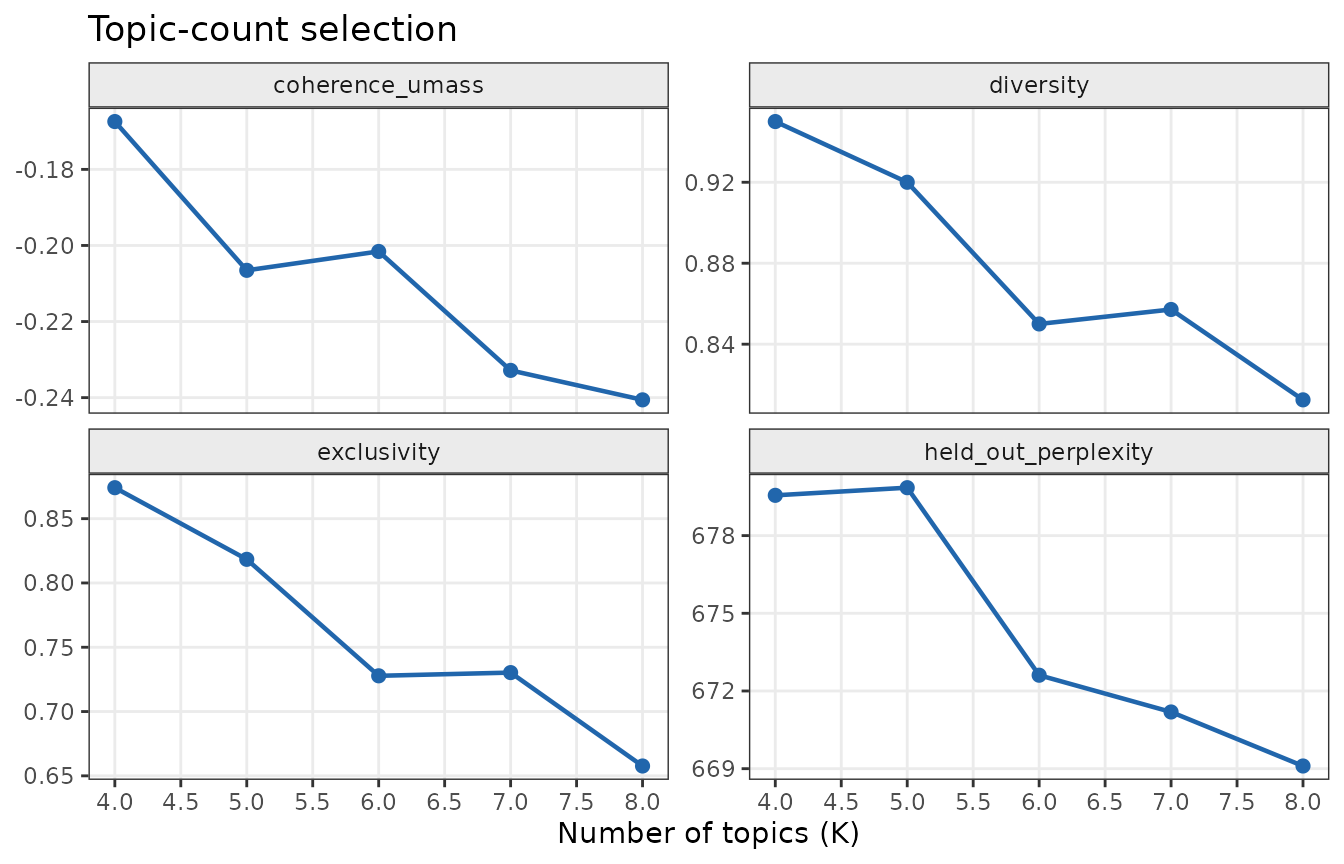

Read these panels together rather than optimizing any one of them. A common pattern is that coherence and exclusivity favor a moderate k while perplexity keeps improving as k grows; the interpretable choice is usually the smallest k that captures the distinct themes without splitting them into redundant near-duplicates.

Evaluate a Chosen Model in Depth

Once the grid points you toward a candidate, refit that single model and inspect it more closely. evaluate_topic_model() returns the same metrics as the grid, but with level = "all" it also reports the per-topic values, which is where you can spot a single incoherent or non-exclusive topic that an aggregate number would hide.

fit <- fit_topic_model(
  dfmat,
  engine  = "topicmodels",
  model   = "lda",
  method  = "Gibbs",
  k       = 6,
  control = list(fit = list(seed = 42L, iter = 400L, burnin = 100L, thin = 1L))
)

evaluation <- evaluate_topic_model(
  fit,
  training = dfmat,
  metrics  = c("coherence_umass", "diversity", "exclusivity"),
  top_n    = 10L,
  level    = "all"
)

evaluation
#>              metric     level topic_id       value supported
#>              <char>    <char>   <char>       <num>    <lgcl>
#>  1: coherence_umass aggregate     <NA> -0.16502170      TRUE
#>  2: coherence_umass     topic Topic001 -0.26043819      TRUE
#>  3: coherence_umass     topic Topic002 -0.20105902      TRUE
#>  4: coherence_umass     topic Topic003 -0.14577500      TRUE
#>  5: coherence_umass     topic Topic004 -0.06337729      TRUE
#>  6: coherence_umass     topic Topic005 -0.23598706      TRUE
#>  7: coherence_umass     topic Topic006 -0.08349362      TRUE
#>  8:       diversity aggregate     <NA>  0.86666667      TRUE
#>  9:     exclusivity aggregate     <NA>  0.74935611      TRUE
#> 10:     exclusivity     topic Topic001  0.79265061      TRUE
#> 11:     exclusivity     topic Topic002  0.66319249      TRUE
#> 12:     exclusivity     topic Topic003  0.81244481      TRUE
#> 13:     exclusivity     topic Topic004  0.59971908      TRUE
#> 14:     exclusivity     topic Topic005  0.87992229      TRUE
#> 15:     exclusivity     topic Topic006  0.74820740      TRUE

It also helps to read the topics themselves. get_top_terms() turns the chosen model into a compact, human-readable view that you can sanity-check against the metrics.

get_top_terms(fit, n = 8, format = "wide")
#>     rank Topic001_term Topic001_prob Topic002_term Topic002_prob Topic003_term
#>    <int>        <char>         <num>        <char>         <num>        <char>
#> 1:     1           can    0.03898137       freedom    0.03771980         world
#> 2:     2          know    0.03134545         human    0.02029819         peace
#> 3:     3           may    0.02409133       liberty    0.01989304          free
#> 4:     4          good    0.02027337           can    0.01948789       nations
#> 5:     5          need    0.01836439       believe    0.01867758        people
#> 6:     6         power    0.01760079          must    0.01827243         earth
#> 7:     7         shall    0.01721900     democracy    0.01705696      strength
#> 8:     8         first    0.01301924       history    0.01584150         faith
#>    Topic003_prob Topic004_term Topic004_prob Topic005_term Topic005_prob
#>            <num>        <char>         <num>        <char>         <num>
#> 1:    0.05761901           new    0.06037910       america    0.03937466
#> 2:    0.04504906           let    0.03872640         every    0.03424330
#> 3:    0.03491201          must    0.03695158       country    0.02945402
#> 4:    0.02964074          work    0.02807752     americans    0.02774357
#> 5:    0.02801881         world    0.02239813      citizens    0.02295430
#> 6:    0.01909821       america    0.02026835      american    0.01953339
#> 7:    0.01869273           can    0.01849354         never    0.01884921
#> 8:    0.01828724        fellow    0.01778361     president    0.01782293
#>    Topic006_term Topic006_prob
#>           <char>         <num>
#> 1:        nation    0.04230236
#> 2:           one    0.03900007
#> 3:        people    0.03635823
#> 4:    government    0.03503732
#> 5:           now    0.02942342
#> 6:      together    0.02612113
#> 7:         years    0.02149792
#> 8:         great    0.02017700

Assess Stability Across Seeds

A model that changes substantially when you change the random seed is hard to defend as a stable research object. assess_topic_stability() makes that check explicit: it refits the same specification across several seeds, aligns vocabularies, matches topics across runs, and reports matched-topic cosine similarities. Because topic labels are arbitrary across runs, the matching step is what makes the comparison meaningful.

stability <- assess_topic_stability(
  dfmat,
  engine  = "topicmodels",
  model   = "lda",
  method  = "Gibbs",
  k       = 6,
  seeds   = 1:4,
  control = list(fit = list(iter = 400L, burnin = 100L, thin = 1L))
)

stability
#> <nlp_topic_stability>
#>   K: 6
#>   runs compared: 3
#>   aggregate stability: 0.6259

Higher matched similarities mean the topic structure is reproducible across seeds. If stability is low at your preferred k, that is useful evidence: it may argue for a smaller k, more iterations, or a more constrained model before the topics are treated as fixed findings.

A Statistical Test for K: OpTop

The metrics and stability checks above are diagnostic, but they still leave the final call to judgment. For a formal decision rule, the OpTop package implements the chi-square optimal-topic test of Lewis and Grossetti (2022). The test compares fitted LDA models against the document-level word distribution and returns a statistical criterion for the optimal number of topics, rather than a metric to eyeball.

NLPstudio does not reimplement the test. Instead it prepares the exact objects OpTop expects and folds the result back into the same selection report. Since OpTop 0.19 the test function is optop_select() (optimal_topic() remains as an alias) and it consumes nlp_topic_fit objects natively - the statistic touches each model only through its fitted word probabilities, so grids may mix fitting methods and even engines, provided every model was fitted on the same corpus and vocabulary. as_optop_input() handles the bookkeeping: it pulls the stored fits out of a select_k_topics(..., return_fits = TRUE) result, orders the grid by K, rejects duplicate topic counts and vocabulary mismatches, and validates and aligns the weighted DFM.

This grid is exactly where the 1.2.0 performance work pays off: parallel grid fitting no longer serializes the training matrix to a worker for every candidate K (each worker now receives it once, and each task ships only its (k, seed) pair), workers cap their thread pools so ncores workers use ncores CPUs, and the per-K evaluation reuses one prepared coherence input across the whole grid. On corpora where the old design was prohibitive, a return_fits = TRUE model grid for OpTop is now practical. When stability checks run in the same call, the opt-in stability_reuse_fit = TRUE reuses each K’s evaluation fit as the first stability run, saving one refit per candidate (the reference run then differs from the default, so numbers change slightly).

selection_vem <- select_k_topics(
  dfmat,
  engine      = "topicmodels",
  model       = "lda",
  method      = "VEM",
  k_grid      = 4:8,
  metrics     = c("diversity", "exclusivity"),
  holdout     = 0,
  return_fits = TRUE,
  control     = list(fit = list(seed = 42L))
)

optop_input <- as_optop_input(
  selection_vem,
  weighted_dfm = as_optop_weighted_dfm(dfmat)
)

optop_result <- OpTop::optop_select(
  topic_models = optop_input$topic_models,
  weighted_dfm = optop_input$weighted_dfm,
  q     = 0.95,
  alpha = 0.05,
  do_plot = FALSE
)

Passing the OpTop output back to summarize_k_selection() merges its columns into the selection report by k, so the statistical test and the interpretability metrics sit in one export-ready table.

k_report_optop <- summarize_k_selection(selection_vem, optop = optop_result)
data.table::fwrite(k_report_optop, tempfile(fileext = ".csv"))

Choosing a Final K

There is no formula that turns this evidence into a single answer, but a defensible workflow looks like this:

Use select_k_topics() to scan a grid and plot() the aggregate metrics to find the region where coherence and exclusivity are strong and diversity has not yet collapsed.
Refit the leading candidates and read their per-topic metrics and top terms with evaluate_topic_model(level = "all") and get_top_terms().
Confirm with assess_topic_stability() that the structure survives a change of seed.
Where a formal criterion is needed, run the OpTop chi-square test and report it alongside the metrics via summarize_k_selection().

The goal is convergent evidence: a k that is coherent, exclusive, non-redundant, stable, and – where you use it – consistent with the statistical test.

API Map

Task	Primary function
Fit a grid of candidate models	`select_k_topics()`
Report selection evidence	`summarize_k_selection()`
Plot metrics against K	`plot()` on the selection object
Evaluate a chosen model	`evaluate_topic_model()`
Read topic top terms	`get_top_terms()`
Assess seed stability	`assess_topic_stability()`
Prepare OpTop inputs	`as_optop_weighted_dfm()`, `as_optop_input()`

References

Aletras, N., & Stevenson, M. (2013). Evaluating topic coherence using distributional semantics. Proceedings of the 14th Conference of the European Chapter of the Association for Computational Linguistics, 13-22.

Lewis, C. M., & Grossetti, F. (2022). A statistical approach for optimal topic model identification. Journal of Machine Learning Research, 23(58), 1-20.

Mimno, D., Wallach, H., Talley, E., Leenders, M., & McCallum, A. (2011). Optimizing semantic coherence in topic models. Proceedings of the 2011 Conference on Empirical Methods in Natural Language Processing, 262-272.

Model Selection, Evaluation, and Stability

by Francesco Grossetti