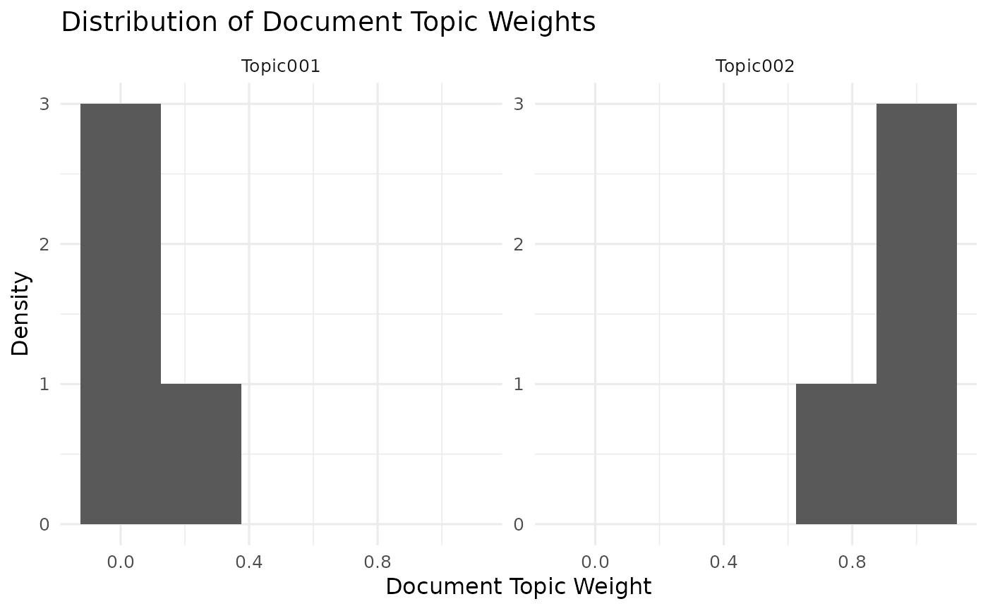
Visualize the distribution of standardized DTW values as faceted histograms, one facet per topic.
Arguments
- x
A supported topic-model object accepted by
get_dtw(), or an already standardized DTW table returned byget_dtw().- topics
Optional topic filter supplied either as numeric indices or as
Topic###identifiers. IfNULL, all topics are plotted.- stat
Character string. Either
"density"(default) or"count".- facet_args
A named list of additional arguments passed to facet_wrap(). Defaults to
list(scales = "free_y").- ...
Additional arguments passed to geom_histogram().
Value
A ggplot object.
Examples
dtm <- methods::as(
  Matrix::Matrix(
    matrix(
      c(1, 0, 1,
        1, 1, 0,
        0, 1, 1,
        1, 1, 1),
      nrow = 4,
      byrow = TRUE
    ),
    sparse = TRUE
  ),
  "dgCMatrix"
)
rownames(dtm) <- paste0("doc", 1:4)
colnames(dtm) <- paste0("term", 1:3)

fit <- fit_topic_model(
  dtm,
  engine = "text2vec",
  model = "lda",
  k = 2,
  control = list(fit = list(n_iter = 25, progressbar = FALSE))
)

plot_dtw(fit, topics = 1:2, bins = 5)