Building augmented data for multi-state models
The msmtools workflow
Francesco Grossetti
francesco.grossetti@unibocconi.it
francesco.grossetti@unibocconi.it
2026-06-05
Source:vignettes/msmtools.Rmd
msmtools.RmdOverview
msmtools prepares longitudinal data for multi-state models fitted with msm (Jackson 2011, 2016). The package exposes four public functions:
-
augment()builds transition-level data from repeated observations; -
polish()removes subjects with incompatible transitions at the same time; -
survplot()compares fitted and empirical survival curves; -
prevplot()compares observed and expected state prevalences.
The examples below use the bundled hosp dataset. It
contains synthetic hospital admissions for 10 subjects.
data(hosp)
hosp[1:6, .(subj, adm_number, gender, age, label_3, dateIN, dateOUT, dateCENS)]
## subj adm_number gender age label_3 dateIN dateOUT dateCENS
## <int> <int> <fctr> <int> <char> <Date> <Date> <Date>
## 1: 1 1 F 83 dead_in 2008-11-30 2008-12-12 2011-04-28
## 2: 1 2 F 83 dead_in 2009-01-26 2009-02-16 2011-04-28
## 3: 1 3 F 83 dead_in 2009-05-13 2009-05-15 2011-04-28
## 4: 1 4 F 83 dead_in 2009-05-20 2009-05-25 2011-04-28
## 5: 1 5 F 83 dead_in 2009-06-12 2009-06-16 2011-04-28
## 6: 1 6 F 83 dead_in 2009-06-20 2009-06-25 2011-04-28Data Augmentation
augment() adds one row per transition endpoint and
creates status variables that can be used directly in an
msm model.
hosp_augmented <- augment(
  data = copy(hosp),
  data_key = subj,
  n_events = adm_number,
  pattern = label_3,
  t_start = dateIN,
  t_end = dateOUT,
  t_cens = dateCENS
)
## Warning in augment(data = copy(hosp), data_key = subj, n_events = adm_number, :
## no t_death has been passed. Assuming that dateCENS contains both censoring and
## death times
hosp_augmented[
  1:8,
  .(subj, adm_number, label_3, augmented, augmented_int, status, status_num)
]
## Key: <subj, adm_number>
## subj adm_number label_3 augmented augmented_int status status_num
## <int> <int> <char> <Date> <int> <char> <int>
## 1: 1 1 dead_in 2008-11-30 14213 IN 1
## 2: 1 1 dead_in 2008-12-12 14225 OUT 2
## 3: 1 2 dead_in 2009-01-26 14270 IN 1
## 4: 1 2 dead_in 2009-02-16 14291 OUT 2
## 5: 1 3 dead_in 2009-05-13 14377 IN 1
## 6: 1 3 dead_in 2009-05-15 14379 OUT 2
## 7: 1 4 dead_in 2009-05-20 14384 IN 1
## 8: 1 4 dead_in 2009-05-25 14389 OUT 2When the input time columns are Date values,
augment() keeps the date-valued transition time and adds an
integer version. This is useful because msm works with
numeric time scales.
names(hosp_augmented)## [1] "subj" "adm_number" "gender" "age"
## [5] "rehab" "it" "rehab_it" "label_2"
## [9] "label_3" "augmented" "augmented_int" "dateIN"
## [13] "dateOUT" "dateCENS" "status" "status_num"
## [17] "n_status"Outcome Schema And Generated States
pattern and state describe different parts
of the augmentation. pattern is the terminal outcome schema
observed in the input data. It can have two values, alive and dead, or
three values, alive, dead during a transition, and dead after a
transition.
state is the generated transition-state vocabulary. It
must always contain three labels: the state at t_start, the
state at t_end, and the absorbing state. This is why a
two-value pattern still needs three state
labels: augment() uses the event times to infer whether
death maps to the absorbing state inside or outside the transition
window.
By default, augment() uses copy = FALSE and
follows data.table by-reference semantics. This avoids
unnecessary memory use on large longitudinal datasets, but the input
object can have its key changed and n_events can be created
when the argument is omitted. Use copy = TRUE when the
original input must remain unchanged.
Duplicate Transition Cleanup
polish() removes entire subjects when different
transitions occur at the same time. The bundled data do not contain such
conflicts, so this call leaves the data unchanged. It also uses
copy = FALSE by default; set copy = TRUE when
the original augmented data should not be keyed or otherwise touched by
reference.
hosp_clean <- polish(
  data = copy(hosp_augmented),
  data_key = subj,
  pattern = label_3
)

nrow(hosp_augmented)
## [1] 114
nrow(hosp_clean)## [1] 114Survival Plot
The plotting helpers work on fitted msm objects.
This example uses a compact three-state transition matrix matching the
default augment() state labels.
Qmat <- matrix(0, nrow = 3, ncol = 3, byrow = TRUE)
Qmat[1, 1:3] <- 1
Qmat[2, 1:3] <- 1
colnames(Qmat) <- c("IN", "OUT", "DEAD")
rownames(Qmat) <- c("IN", "OUT", "DEAD")

msm_model <- msm(
  status_num ~ augmented_int,
  subject = subj,
  data = hosp_augmented,
  exacttimes = TRUE,
  gen.inits = TRUE,
  qmatrix = Qmat,
  method = "BFGS",
  control = list(fnscale = 6e+05, trace = 0, REPORT = 1, maxit = 10000)
)
surv_p <- survplot(msm_model, km = TRUE, grid = 10)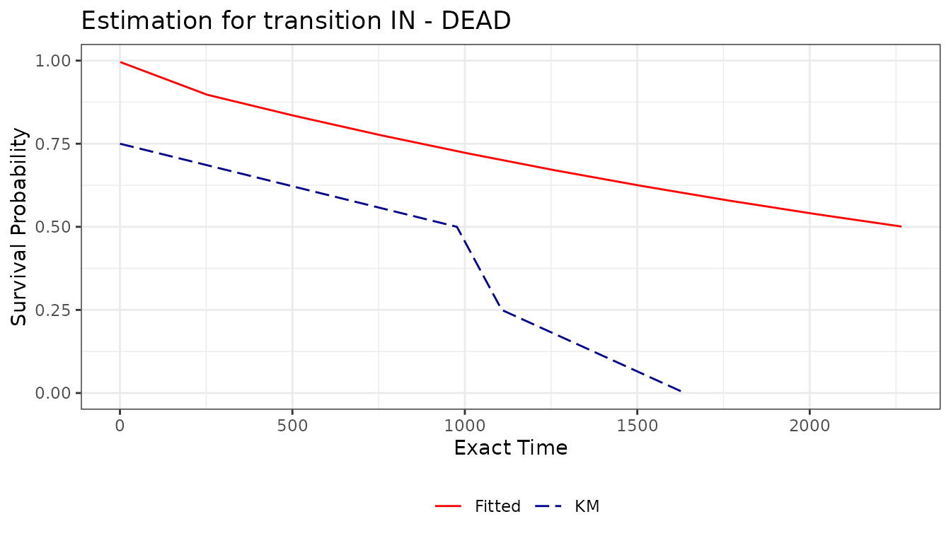
surv_p
The fitted and Kaplan-Meier data tables are attached to the plot as
named fields, accessible with the standard $ operator:
surv_p$fitted[1:6]## time surv
## <num> <num>
## 1: 1.0 0.9957174
## 2: 252.7 0.8974193
## 3: 504.4 0.8343219
## 4: 756.1 0.7756608
## 5: 1007.8 0.7211242
## 6: 1259.5 0.6704220
surv_p$km[1:6]## subject time time_exact anystate km
## <int> <int> <int> <num> <num>
## 1: 5 13985 0 1 0.75
## 2: 6 14962 977 1 0.50
## 3: 1 15092 1107 1 0.25
## 4: 7 15623 1638 1 0.00
## 5: NA NA NA NA NA
## 6: NA NA NA NA NAPrevalence Plot
prevplot() uses the output of
msm::prevalence.msm() and returns a ggplot
object.
prev <- prevalence.msm(
  msm_model,
  covariates = "mean",
  ci = "normal",
  times = seq(
    min(hosp_augmented$augmented_int),
    max(hosp_augmented$augmented_int),
    length.out = 6
  )
)

prev_p <- prevplot(msm_model, prev, ci = TRUE, M = FALSE)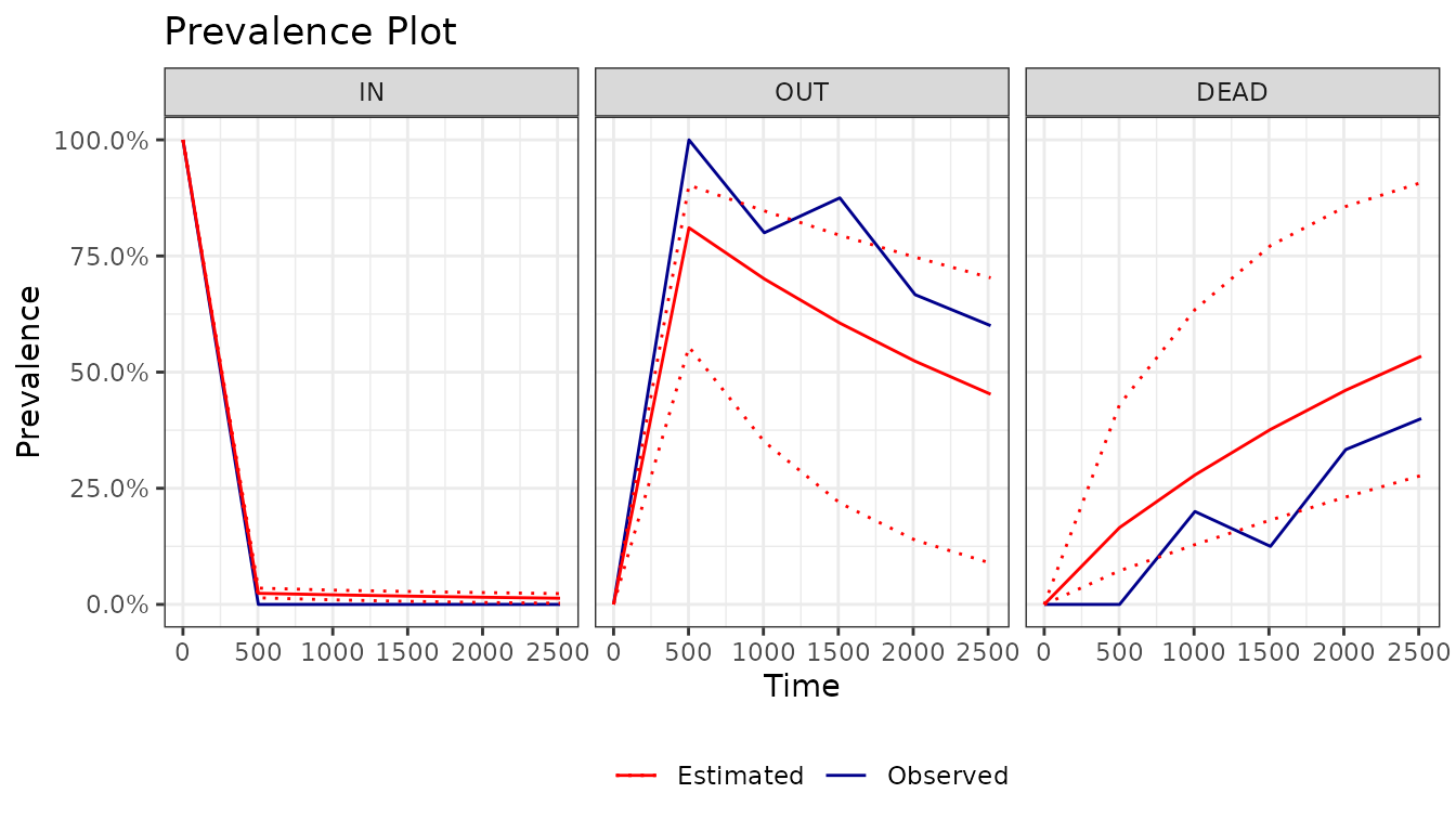
prev_p
The long-format prevalence data used to build the plot is attached as
$prevalence:
prev_p$prevalence[1:6]## time state obs hat lwr upr
## <int> <fctr> <num> <num> <num> <num>
## 1: 0 IN 1 1.00000000 1.000000000 1.00000000
## 2: 503 IN 0 0.02390625 0.014228910 0.03510729
## 3: 1006 IN 0 0.02066274 0.009834560 0.03072290
## 4: 1510 IN 0 0.01785929 0.006561754 0.02785672
## 5: 2013 IN 0 0.01543621 0.004145471 0.02546796
## 6: 2517 IN 0 0.01334188 0.002612084 0.02328773Notes
The current 2.x series keeps the public API stable while modernizing
dependencies, documentation, tests, and CI. Larger internal changes to
augment() are intentionally deferred until after the
maintenance releases.