Plot a held-out validation result

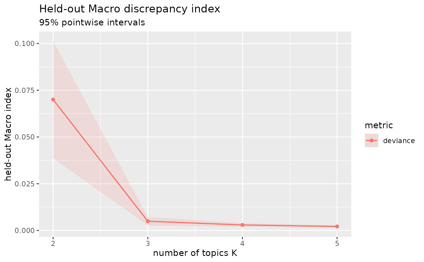
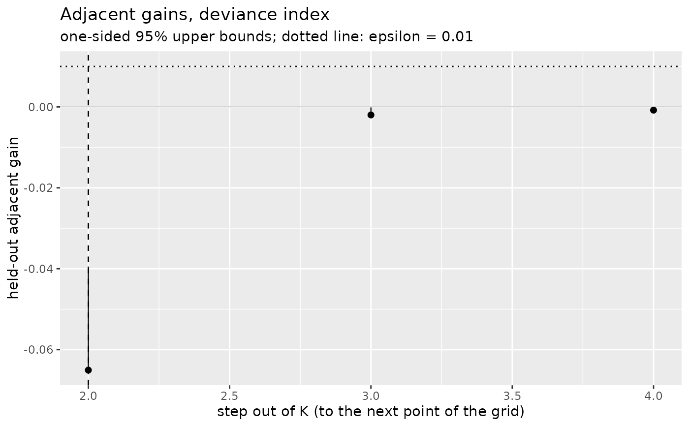
Visualize an optop_index_holdout() result. The "macro" view draws the held-out Macro index against the number of topics for every evaluated metric, with its confidence band: the working view for locating where the curve flattens. The "gains" view draws the adjacent paired gains of one metric with their one-sided upper bounds and the epsilon-adequacy rule of optop_gain_table(): the first step out of K whose upper bound falls below epsilon selects K, marked by the dashed vertical line.

Usage

# S3 method for class 'optop_holdout'
plot(
  x,
  which = c("macro", "gains"),
  metric = NULL,
  epsilon = 0.01,
  alpha = 0.05,
  ...
)

Arguments

x

An optop_index_holdout() result.

which

"macro" (default) or "gains".

metric

For the gains view, the metric to draw (default: the first evaluated metric); the macro view always draws all of them.

epsilon, alpha

The adequacy tolerance and the one-sided level of the gains view, passed to optop_gain_table().

...

Ignored.

Value

The ggplot object, invisibly (the plot is drawn as a side effect).

Examples

# \donttest{
# simulate a corpus with known truth and split train/eval
rdirich <- function(n, k) {
  g <- matrix(stats::rgamma(n * k, shape = 1), n, k)
  g / rowSums(g)
}
theta <- rdirich(60, 3)
phi <- rdirich(3, 120)
colnames(phi) <- sprintf("w%03d", 1:120)
dtm <- sim_dfm(theta, phi, doc_length = 150, seed = 7)

split <- seq_len(40)
models <- lapply(2:5, function(k) {
  topicmodels::LDA(quanteda::convert(dtm[split, ], to = "topicmodels"),
                   k = k, method = "VEM",
                   control = list(seed = 500 + k))
})
baseline <- optop_make_baseline(dtm[split, ])
ho <- optop_index_holdout(models, dtm[-split, ], baseline,
                          metrics = "deviance")
plot(ho)

plot(ho, which = "gains", epsilon = 0.01)

# }