Working With OpTop
Parametric Tests and Discrepancy Indices for Topic Models
Francesco Grossetti
July 6, 2026
Source:vignettes/OpTop.Rmd
OpTop.RmdOpTop implements the parametric tests of Lewis and Grossetti (2022, JMLR 23(58)) for identifying the optimal number of topics of a Latent Dirichlet Allocation (LDA) model, together with a family of regression-style goodness-of-fit (GoF) indices. This vignette illustrates both on the corpus of the paper’s case study and concludes with a simulation study in which the true number of topics is known.
The only step performed offline is the estimation of the LDA models:
100 fits on the full corpus and 30 fits on the training split of the
held-out analysis. Everything downstream, from every
optop_select() call to each table, figure, and number
quoted in the text, is computed from those fits.
Setting Up: Corpus, Grid, Models
We use the U.S. Presidential Inaugural Address corpus distributed with quanteda, the same corpus analyzed in the paper’s case study, with a standard preprocessing pipeline and a vocabulary trim. The grid spans K = 2 to 200 in steps of 2.
library(OpTop)

ncores <- 6

# Tokenize
toks <- quanteda::data_corpus_inaugural |>
  quanteda::tokens(remove_punct = TRUE,
                   remove_symbols = TRUE,
                   remove_numbers = TRUE) |>
  quanteda::tokens_tolower() |>
  quanteda::tokens_remove(quanteda::stopwords())

# Create DFM (with raw counts as well as proportions)
mydfm        <- quanteda::dfm(toks)
mydfm_sub    <- quanteda::dfm_trim(mydfm, min_termfreq = 5)
weighted_dfm <- quanteda::dfm_weight(mydfm_sub, scheme = "prop")

K_grid <- seq(2, 200, by = 2)

# Estimate VEM models in parallel
VEM_models <- parallel::mclapply(
  K_grid,
  function(k) {
    message("Estimating LDA with K = ", k)
    topicmodels::LDA(x = mydfm_sub, k = k)
  },
  mc.cores = ncores
)
After trimming, the corpus has 60 documents and 2654 features (down from 9359). The VEM fits above are unseeded, so re-running the pipeline may alter individual statistics slightly; the numbers quoted in this vignette come from one such run.
The Test 1 Statistic
The test evaluates overall model adequacy: how well a K-topic model explains the corpus. It relies on the multinomial structure that LDA itself assumes. A fitted K-topic model describes document j by a vector of document-topic weights \theta_j^K and each topic by a distribution over the P vocabulary words, collected in the topic-word matrix \phi^K. The model’s fitted probability of word p in document j is
I_{jp}^{K} = \sum_{k=1}^{K} \theta_{jk}^{K}\,\phi_{kp}^{K}, \tag{1}
which is Equation 5 in the paper. Equation 4 of the paper represents the observed word-proportion vector d_j as this fitted distribution plus multinomial sampling noise. If the K-topic model fully characterizes the corpus, one would be unable to reject the hypothesis that the observed and estimated word distributions are statistically indistinct: a classical goodness-of-fit situation.
Because a large number of words carry near-zero fitted probability, the comparison is made on a per-document envelope. The fitted probabilities I_{jp}^K are sorted in decreasing order and the smallest leading set whose cumulative mass exceeds q is retained; these are the P_j relatively important words of document j. The remaining, relatively unimportant words are collapsed into a single bin (the paper’s Equations 6 and 7). With the words of document j indexed in decreasing order of I_{jp}^K, the fitted and observed masses of that bin are
I^{K}_{j,\min} = \sum_{p = P_j + 1}^{P} I^{K}_{jp} \;<\; 1 - q, \tag{2a}
D_{j,\min} = \sum_{p = P_j + 1}^{P} D_{jp}. \tag{2b}
Collapsing the relatively unimportant words in this manner preserves
the underlying multinomial assumption. Note that the basis for the
cutoff is the fitted model rather than the observed documents; the
paper’s numerical setting I^K = 0.05
corresponds to q = 0.95. Test 1 (Equation 8 of the paper)
then aggregates the Pearson discrepancies over documents:
\mathrm{OpTop}_J^K = \sum_{j=1}^{J} \left[\, (P_j + 1) \left( \sum_{p=1}^{P_j} \frac{\bigl(D_{jp} - I_{jp}^K\bigr)^2}{I_{jp}^K} +\; \frac{\bigl(D_{j,\min} - I_{j,\min}^K\bigr)^2}{I_{j,\min}^K} \right) \right] \sim \chi^2_{P_J}, \tag{3}
where \mathrm{OpTop}_J^K is
distributed chi-square with P_J =
\sum_{j=1}^{J} P_j degrees of freedom. Misspecification, that is
a K too coarse to reproduce the word
distributions, can only inflate the statistic, so evidence against
adequacy is found in the upper tail. The package reports the
standardized statistic \mathrm{OpTop}_J^K / P_J (the version plotted
in the paper’s Figure 2, which fluctuates around 1 under an adequate
model) in the OpTop column, the degrees of freedom P_J in df, and the upper-tail
p-value in pval.
Running the Test
optop_select() consumes word proportions
(weighted_dfm above), while the discrepancy indices of the
second part consume the raw counts; both objects are therefore
required. With verbose = TRUE, the function reports its
setup, its progress across the grid, the selected model together with
the rule that chose it, and the elapsed time:
# Use the sequential approach
chi_seq <- optop_select(topic_models = VEM_models,
                        weighted_dfm = weighted_dfm,
                        selection = "sequential",
                        q = 0.95,
                        alpha = 0.01,
                        do_plot = FALSE)
#> ── Optimal topic selection ──
#> Loading required namespace: topicmodels
#> ℹ Evaluating 100 models on 60 documents and 2654 features (q = 0.95, alpha = 0.01, selection = sequential)
#> ✔ Optimal model has 34 topics (selected by sequential adequacy scan at alpha = 0.01)
#> ℹ Completed in 0.93s
# Use the global minimum approach
chi_min <- optop_select(topic_models = VEM_models,
                        weighted_dfm = weighted_dfm,
                        selection = "min",
                        q = 0.95,
                        alpha = 0.01,
                        do_plot = FALSE)
#> ── Optimal topic selection ──
#> ℹ Evaluating 100 models on 60 documents and 2654 features (q = 0.95, alpha = 0.01, selection = min)
#> ✔ Optimal model has 96 topics (selected by global minimum)
#> ℹ Completed in 0.7sReading the Result
optop_select() returns a data.table with
one row per model:
head(chi_seq)
#>    topic    OpTop     df  pval
#>    <num>    <num>  <num> <num>
#> 1:     2 4.495543 127613     0
#> 2:     4 3.093535  93766     0
#> 3:     6 2.707646  85074     0
#> 4:     8 2.513613  79078     0
#> 5:    10 2.313265  74733     0
#> 6: 12 2.131487 71409 0-
OpTopis the standardized Test 1 statistic, the raw chi-square of Equation (3) divided by its degrees of freedom, and the quantity plotted in the paper’s Figure 2. Under an adequate model it fluctuates around 1. -
dfis P_J = \sum_j P_j, the total number of relatively important words across documents. -
pvalis the upper-tail p-value of the raw statistic. Small values indicate that the observed discrepancy is larger than sampling noise can explain, so the K-topic model is rejected.
The selection rule affects which K is reported
as optimal (and the plot guides), never the table itself. The two calls
above return identical tables:
all.equal(chi_seq, chi_min)
#> [1] TRUE
The Two Selection Rules
Both rules are direct computations on the returned table and can be stated explicitly:
alpha <- 0.01

# "sequential": the smallest K the test fails to reject
seq_pick <- chi_seq[pval > alpha, topic][1]

# "min": the K with the minimum standardized statistic
min_pick <- chi_seq[which.min(OpTop), topic]

c(sequential = seq_pick, min = min_pick)
#> sequential        min
#>         34         96
selection = "sequential" implements the
classical sequential scan for model order: K is increased until the first model the test
fails to reject (pval > alpha). The rationale
is parsimony: the rule selects the smallest K that the data cannot distinguish from
adequate. On this corpus the sequential rule selects K =
34. If every model were rejected, optop_select()
would fall back to the global minimum with a warning.
selection = "min" reproduces the
published case study: the optimum is identified as the K-topic model with the minimum standardized
statistic across the grid. Here the minimum is at K =
96, close to the 92 topics the paper identifies on the
untrimmed vocabulary of the same corpus and, as the sweep below shows,
insensitive to the choice of q. One practical remark is in
order: the minimum rule requires a grid that extends beyond the
flattening of the curve. On a grid truncated at K = 100 the minimum sits
at the boundary, and only the full scan up to K = 200 allows it to
stabilize. The behavior has a structural explanation. The
df column decreases steadily with K because the envelopes shrink as the fitted
distributions concentrate, and since the null level of the standardized
statistic scales with the envelope size, part of the curve’s long
decline reflects envelope shrinkage rather than genuine improvement in
fit. The calibrated p-values of the next section absorb this effect
automatically; the raw curve does not. The sequential rule, by
construction, stops at the first adequate K and is unaffected by the extent of the
grid.
The p-value column explains when and why the two rules diverge:
summary(chi_seq$pval)
#>    Min. 1st Qu.  Median    Mean 3rd Qu.    Max.
#>    0.00    1.00    1.00    0.83    1.00    1.00
With df of the order of 27,764, the chi-square reference
distribution is extremely concentrated, so p-values saturate: models
whose standardized statistic is materially above 1 receive p-values of
essentially 0, and models at or below 1 receive p-values of essentially
1. When every model is rejected, the sequential rule falls back to the
global minimum with a warning; when several models are accepted, it
stops at the smallest, which may precede the minimum by a wide margin.
This is a documented calibration caveat of the chi-square reference (see
?optop_select): in saturated regimes the information is
carried by the shape of the OpTop curve and by its
minimum.
Because the return value is a table, custom figures follow directly:
ggplot(chi_seq, aes(x = topic, y = OpTop)) +
  geom_line(linewidth = 0.8, color = "royalblue") +
  geom_vline(xintercept = seq_pick, linetype = 2) +
  geom_vline(xintercept = min_pick, linetype = 3) +
  annotate("point", x = min_pick, y = min(chi_seq$OpTop),
           color = "red", shape = 4, size = 4) +
  labs(x = "Topics", y = expression(OpTop[J]^{K}),
       title = "Standardized Test 1 statistic across the grid",
       subtitle = sprintf("sequential pick: K = %d (dashed) | global minimum: K = %d (dotted)",
                          seq_pick, min_pick)) +
  theme_bw()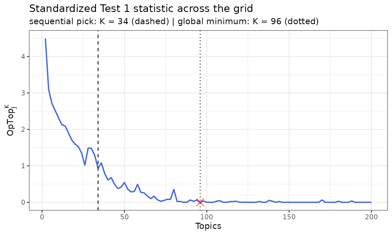
Calibrated p-Values
The saturation above has a precise cause: the \chi^2_{P_J} reference is an asymptotic guide rather than the exact null law of the statistic. Write k_j = P_j + 1 for the number of envelope bins of document j and N_j for its length in tokens. The classical Pearson statistic on counts, X^2_j = N_j \sum_b (d_{jb} - p_{jb})^2 / p_{jb}, is the object with the textbook \chi^2_{k_j - 1} asymptotics; the document term of Equation (3) is instead
S_j = (P_j + 1) \sum_b \frac{(d_{jb} - p_{jb})^2}{p_{jb}} = \frac{k_j}{N_j}\, X^2_j , \tag{4}
which differs from the calibrated object by the factor k_j / N_j. In addition, the fitted probabilities are estimated from the same data they are tested against. Calibration therefore replaces the \chi^2 reference with the distribution of T = \sum_j S_j under the conditional fitted-model null
c_j \sim \mathrm{Multinomial}\bigl(N_j,\; I_j^K\bigr), \qquad j = 1, \dots, J, \tag{5}
with \hat\theta and \hat\phi held fixed at their estimates. Two properties make this exact and fast: the envelope depends only on the model, never on the data, and a multinomial collapsed over bins is multinomial on the collapsed probabilities. The null replicates can therefore be drawn directly on the k_j bins p_j = (I^K_{j1}, \dots, I^K_{jP_j}, I^K_{j,\min}), which is equivalent to simulating entire documents over the vocabulary at a small fraction of the cost. The only new ingredient the user supplies is the vector of document lengths N_j:
doc_lens <- quanteda::ntoken(mydfm_sub)

chi_cal <- optop_select(topic_models = VEM_models,
                        weighted_dfm = weighted_dfm,
                        q = 0.95,
                        alpha = 0.01,
                        calibrate = "bootstrap",
                        n_boot = 200,
                        doc_lengths = doc_lens,
                        seed = 20260703,
                        do_plot = FALSE)
#> ── Optimal topic selection ──
#> ℹ Evaluating 100 models on 60 documents and 2654 features (q = 0.95, alpha = 0.01, selection = sequential)
#> ℹ Calibrating p-values by parametric bootstrap (B = 200, seed = 20260703) under the fitted-model null
#> ✔ Optimal model has 8 topics (selected by sequential adequacy scan at alpha = 0.01, bootstrap-calibrated)
#> ℹ Completed in 46.83sWith calibrate = "bootstrap", B = n_boot null replicates T^{*}_1, \dots, T^{*}_B are drawn as above
and the reported p-value is the empirical upper tail with the standard
finite-sample correction,
\hat{p} = \frac{1 + \#\{\, b : T^{*}_b \ge T \,\}}{B + 1}, \tag{6}
so alpha is a genuine Type-I error rate with respect to
the conditional null, at resolution 1/(B+1). The bootstrap is the most expensive
stage of the pipeline; its cost, and the effect of the
n_threads argument, are quantified in the section A Note On Computational
Efficiency. The table now carries two p-value columns:
pval (the calibrated value used by the selection rules) and
pval_chisq (the asymptotic value, kept for comparison):
head(chi_cal)
#>    topic    OpTop     df        pval pval_chisq
#>    <num>    <num>  <num>       <num>      <num>
#> 1:     2 4.495543 127613 0.004975124          0
#> 2:     4 3.093535  93766 0.004975124          0
#> 3:     6 2.707646  85074 0.004975124          0
#> 4:     8 2.513613  79078 0.119402985          0
#> 5:    10 2.313265  74733 0.004975124          0
#> 6:    12 2.131487  71409 0.014925373          0
The bootstrap is the reference method;
calibrate = "moment" targets the same null in closed form.
Haldane (1937) gives the exact multinomial moments of the count-based
Pearson statistic over k_j bins:
\mathrm{E}\bigl[X^2_j\bigr] = k_j - 1, \tag{7a}
\begin{split} \mathrm{Var}\bigl[X^2_j\bigr] &= 2(k_j - 1) \\ &\quad + \frac{\sum_b 1/p_{jb} - k_j^2 - 2k_j + 2}{N_j}. \end{split} \tag{7b}
Since S_j = (k_j/N_j)\,X^2_j and documents are independent, the null mean and variance of T follow by scaling and summing, \mu = \sum_j (k_j/N_j)(k_j - 1) and \sigma^2 = \sum_j (k_j/N_j)^2\,\mathrm{Var}[X^2_j], and the reference is the Satterthwaite scaled chi-square matching them:
\begin{gathered} T \overset{\text{approx}}{\sim} a\,\chi^2_\nu, \qquad a = \frac{\sigma^2}{2\mu}, \qquad \nu = \frac{2\mu^2}{\sigma^2}, \\ \hat{p} = \Pr\!\left(\chi^2_\nu \ge T/a\right). \end{gathered} \tag{8}
The method requires no simulation and no seed; it is a fast approximation that corrects the location and the scale of the reference, although not its higher moments:
chi_cal_mm <- optop_select(topic_models = VEM_models,
                           weighted_dfm = weighted_dfm,
                           q = 0.95,
                           alpha = 0.01,
                           calibrate = "moment",
                           doc_lengths = doc_lens,
                           do_plot = FALSE)
#> ── Optimal topic selection ──
#> ℹ Evaluating 100 models on 60 documents and 2654 features (q = 0.95, alpha = 0.01, selection = sequential)
#> ℹ Calibrating p-values by moment matching (Satterthwaite scaled chi-square) under the fitted-model null
#> ✔ Optimal model has 8 topics (selected by sequential adequacy scan at alpha = 0.01, moment-calibrated)
#> ℹ Completed in 0.79sThe following figure compares the three reference distributions:
pv <- melt(
  data.table(topic = chi_cal$topic,
             `chi-square` = chi_cal$pval_chisq,
             bootstrap = chi_cal$pval,
             moment = chi_cal_mm$pval),
  id.vars = "topic", variable.name = "reference", value.name = "pvalue"
)

ggplot(pv, aes(x = topic, y = pvalue, color = reference)) +
  geom_line(linewidth = 0.7) +
  geom_hline(yintercept = alpha, linetype = 3) +
  labs(x = "Topics", y = "p-value",
       title = "P-values under the three reference distributions",
       subtitle = sprintf("dotted line: alpha = %.2f", alpha)) +
  theme_bw()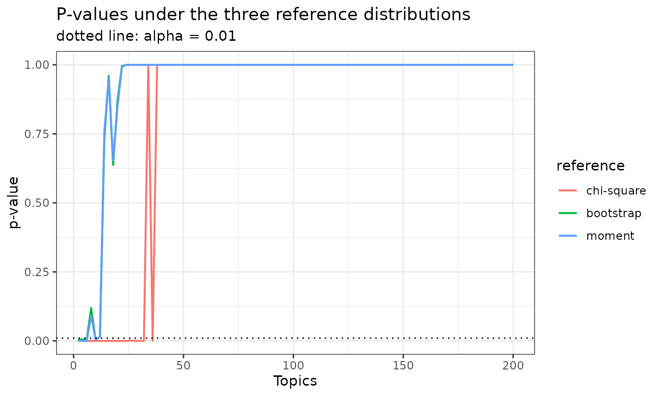
Because the p-values themselves do not depend on alpha,
the conventional thresholds can be scanned directly on the tables
already computed:
alphas <- c(0.01, 0.05, 0.10)

picks_alpha <- data.table(
  alpha = alphas,
  bootstrap = sapply(alphas, function(a) chi_cal[pval > a, topic][1]),
  moment = sapply(alphas, function(a) chi_cal_mm[pval > a, topic][1]),
  `chi-square` = sapply(alphas, function(a) chi_seq[pval > a, topic][1])
)

knitr::kable(picks_alpha,
caption = "Sequential pick by reference distribution as alpha varies")| alpha | bootstrap | moment | chi-square |
|---|---|---|---|
| 0.01 | 8 | 8 | 34 |
| 0.05 | 8 | 8 | 34 |
| 0.10 | 8 | 14 | 34 |
Interpretation follows from the null the calibration targets. The
calibrated sequential pick answers a precise question: what is the
smallest K whose residual discrepancy
could plausibly be produced by multinomial sampling noise alone, if the
fitted model were the truth? On this corpus this happens already at
K = 8. The fit does continue to improve beyond that point, since the
OpTop curve decreases until its minimum at K = 96, but from
there onward the improvements are smaller than what sampling noise can
account for at the chosen alpha.
The uncalibrated scan is best understood as a reduced-chi-square
heuristic. With df this large the asymptotic p-values
saturate at 0 or 1, so in practice the rule stops at the first K whose standardized discrepancy falls below
1. This is a reasonable descriptive criterion, but its implicit
threshold is not tied to the actual null level of the statistic. On this
corpus the bootstrap places that null level closer to 2 than to 1, so
the heuristic demands more than noise-level adequacy and stops later, at
K = 34. The selection is also unstable: on this grid the next model, K =
36, is rejected again, and the sweep of q below moves the
pick from 20 to 38. When the implicit threshold happens to lie close to
the true null level, the same heuristic performs well; the simulation
study at the end of this vignette, where the ground truth is known, is
such a case. What calibration adds is therefore not a different answer
but a guarantee. Raising alpha demands stronger evidence of
adequacy, so the pick moves weakly upward, as the table shows, and
alpha becomes a genuine Type-I error rate with respect to
the fitted-model null, at bootstrap resolution
1 / (n_boot + 1). In summary, the calibrated sequential
rule identifies the most parsimonious statistically adequate
K, while the global-minimum rule and
the discrepancy indices below quantify maximal descriptive fit.
The two questions are distinct.
One caveat applies to both calibrations: they hold the estimated
theta and phi fixed, so they do not account
for estimation noise in the LDA parameters themselves (see
?optop_select).
The Role of q
q controls the per-document envelope introduced in
Equations (2a) and (2b): the fitted word probabilities are sorted in
decreasing order and the smallest leading set whose cumulative mass
exceeds q is retained, while the relatively unimportant
words are collapsed into a single bin whose mass remains strictly below
1 - q. In the paper’s notation q = 1 - I^K,
and its numerical setting I^K = 0.05 corresponds to the
default q = 0.95.
Re-running the test across a sweep of q values is a
direct sensitivity check:
q_grid <- c(0.80, 0.90, 0.95, 0.99)

chi_by_q <- lapply(q_grid, function(q) {
  optop_select(VEM_models, weighted_dfm, q = q, alpha = alpha,
               do_plot = FALSE)
})
names(chi_by_q) <- sprintf("q%.2f", q_grid)
q_curves <- rbindlist(
  lapply(names(chi_by_q), function(nm) {
    data.table(q = as.numeric(sub("q", "", nm)), chi_by_q[[nm]])
  })
)

ggplot(q_curves, aes(x = topic, y = OpTop, color = factor(q))) +
  geom_line(linewidth = 0.7) +
  labs(x = "Topics", y = expression(OpTop[J]^{K}), color = "q",
       title = "Standardized Test 1 statistic across the q sweep") +
  theme_bw()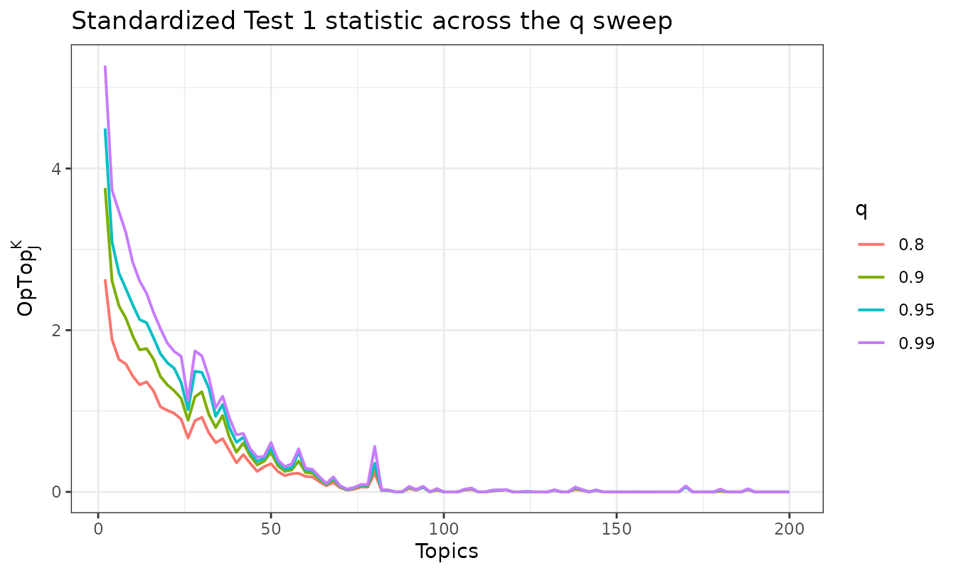
Applying the two selection rules to each element of the sweep shows
how the selected K responds to
q:
picks_by_q <- data.table(
  q = as.numeric(sub("q", "", names(chi_by_q))),
  sequential = sapply(chi_by_q, function(tab) tab[pval > alpha, topic][1]),
  min = sapply(chi_by_q, function(tab) tab[which.min(OpTop), topic])
)

knitr::kable(picks_by_q, caption = "Selected K by rule as q varies")| q | sequential | min |
|---|---|---|
| 0.80 | 20 | 96 |
| 0.90 | 26 | 96 |
| 0.95 | 34 | 96 |
| 0.99 | 38 | 96 |
Larger q retains more words per document, so the degrees
of freedom grow and the envelope covers more of each document’s
distribution, while smaller q makes the comparison coarser
and computationally cheaper. The sequential pick moves with
q, whereas the global minimum is unaffected. The default
q = 0.95 follows the paper.
Goodness-of-Fit: The Discrepancy Indices
The second family of tools asks a complementary question: not
which K is optimal but how much of the word-count structure
a given model explains. Following Lewis and Grossetti (2026), each
index measures the proportional reduction in discrepancy achieved by a
K-topic model relative to the no-topics
baseline in which every document follows the corpus word distribution.
The comparison is carried out on a harmonized support:
a fixed, document-specific set of rare words, computed as a union over
the whole model grid and the baseline, is collapsed so that
every K is evaluated on the same bins.
Because the harmonized set depends on the grid and on the threshold
constant c, indices are comparable across studies only
under a common pair; the default c = 1 follows the paper’s
recommendation for deviance-primary work. The indices consume raw
counts:
dtm_counts <- methods::as(mydfm_sub, "CsparseMatrix")
partition <- optop_make_partition(VEM_models, dtm_counts, c = 1)
baseline <- optop_make_baseline(dtm_counts)

idx_tab <- optop_index_table(VEM_models, dtm_counts,
                             metrics = c("se", "chisq", "deviance"),
                             partition = partition, baseline = baseline,
                             macro = TRUE)
idx <- melt(idx_tab,
            id.vars = "K",
            measure.vars = c("R2_SE", "R2_chisq", "R2_dev"),
            variable.name = "metric", value.name = "R2")

ggplot(idx, aes(x = K, y = R2, color = metric)) +
  geom_line(linewidth = 0.7) +
  labs(x = "Topics", y = expression(R^2),
       title = "Discrepancy indices across the grid (document level, micro)") +
  theme_bw()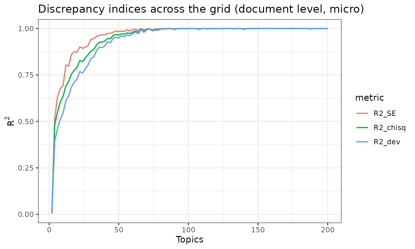
All three indices are regression-style R-squared analogues: 0 indicates that the model explains no more than the corpus-wide baseline, and 1 indicates a perfect account of the harmonized word counts. The deviance index is bounded above by one, while the Pearson and squared-error indices are not confined to [0, 1]; a negative value is informative, since it indicates that the fitted model performs worse than the baseline under that discrepancy. The indices typically rise steeply at small K and flatten once additional topics no longer provide significant incremental explanatory power; the region where the curves flatten corresponds to the neighborhood in which Test 1 locates the optimum. These full-corpus values are descriptive summaries of in-sample fit and should not be the sole basis for choosing K.
The indices are also available at the word level, computed on the unbinned vocabulary, which serves as a diagnostic: it identifies the words the selected model captures well and those it misses. For the deviance family this diagnostic is in-sample by construction: its null side is exact only against the unsmoothed corpus baseline of the counts being scored, and since 0.20.1 the package warns when a different baseline is supplied, because the resulting values are not a valid held-out deviance. For the sequential pick (K = 34), the micro word-level chi-square index is 0.867; the ten highest- and lowest-index words are reported below:
knitr::kable(
  data.frame(
    `best words` = names(word_r2$best),
    R2_best = round(unname(word_r2$best), 3),
    `worst words` = names(word_r2$worst),
    R2_worst = round(unname(word_r2$worst), 3),
    check.names = FALSE
  ),
  caption = sprintf("Word-level chi-square R2 at K = %d: the ten best and worst captured words",
                    word_r2$k)
)| best words | R2_best | worst words | R2_worst |
|---|---|---|---|
| aggregate | 1 | basic | -0.007 |
| statutes | 1 | rights | 0.296 |
| enactment | 1 | called | 0.353 |
| whatsoever | 1 | law | 0.408 |
| revision | 1 | form | 0.454 |
| operations | 1 | fulfillment | 0.458 |
| roman | 1 | without | 0.474 |
| interstate | 1 | already | 0.494 |
| type | 1 | safe | 0.528 |
| eighteenth | 1 | many | 0.535 |
The Null-Discrepancy Floor
Each document-level index is a ratio, and its denominator is itself a measured quantity: the discrepancy of the no-topics baseline on that document. For almost every document the denominator is comfortably large. The exception is a document whose entire support is rare relative to its length: at partition resolution every one of its words falls into the collapsed min bin, and there the observed bin mass equals the baseline bin mass by construction. The baseline discrepancy is then numerically zero in every family at once, and the ratio degenerates; such a document contributes an arbitrarily wild value to the Macro average while carrying no usable information about fit.
The index functions therefore restrict the Macro aggregation to the
documents whose baseline discrepancy clears a floor, D_j(\mathrm{null}) \ge min_null,
and report every exclusion. The default floor is the partition constant
c, the same yardstick that defines the harmonized support:
a discrepancy below the resolution of a single expected count is
indistinguishable from rounding noise. Setting min_null = 0
restores the strict-positivity rule of versions before 0.14.1
exactly.
dev_floor <- optop_index_deviance(m_star, dtm_counts, partition, baseline,
                                  macro = TRUE)
dev_floor$n_null_excluded
The inaugural corpus is not a contrived example. At the sequential pick (K = 34) the floor excludes 1 speech (1.7% of the corpus): 1793-Washington, Washington’s famously brief second inaugural, 53 tokens after preprocessing. Every one of its surviving words is rare at the partition resolution \tau_j = c / L_j, the whole document lives in the collapsed min bin, and its baseline deviance evaluates to exactly 0: the ratio is 0/0 and carries no information about fit. The Macro index over the remaining speeches is 0.7901.
The strict-positivity rule of versions before 0.14.1 happens to drop an exact zero as well, but silently, and only by the sign luck of floating-point arithmetic: a collapsed document landing a hair above zero would have stayed in, free to contribute a ratio in the thousands to the Macro average. The floor replaces that accident with a rule stated in the units of the analysis (one expected count) and reports every exclusion through the accompanying alert, so a silent change of estimand can never happen. The Micro index is nearly immune either way: its weights are proportional to the baseline discrepancies, so a near-collapsed document has almost no say in it.
Held-Out Validation and Topic-Number Choice
The indices above are computed on the same documents used to estimate the models, so they describe in-sample fit and are optimistic by construction: every additional topic gives the model more freedom to adapt to the estimation sample, whether or not the gain reflects structure that generalizes. Formal inference on fit, and a topic-number choice that can be defended statistically, require documents the models have never seen (Lewis and Grossetti, 2026).
We therefore hold out 15 of the 60 speeches, chosen at random under a fixed seed, and refit the grid on the remaining 45 alone, for K = 2 to 60 in steps of 2. The vocabulary is fixed by the training split; the 7 word types that occur only in held-out speeches (about 0.4% of the evaluation tokens) are collapsed into a synthetic out-of-vocabulary bin that every model treats as rare. The corpus baseline is likewise estimated on the training split, so nothing in the evaluation documents influences the fitted models or the targets they are compared against.
set.seed(20260709)
n_docs <- quanteda::ndoc(mydfm_sub)
eval_idx <- sort(sample(n_docs, round(0.25 * n_docs)))
dfm_eval <- mydfm_sub[eval_idx, ]
dfm_train <- quanteda::dfm_trim(mydfm_sub[-eval_idx, ], min_termfreq = 1)

VEM_train <- lapply(seq(2, 60, by = 2), function(k) {
  topicmodels::LDA(x = dfm_train, k = k, control = list(seed = 500 + k))
})

base_train <- optop_make_baseline(dfm_train)
ho <- optop_index_holdout(VEM_train, dfm_eval, base_train)
optop_index_holdout() gives each evaluation document its
topic weights under the trained topics held fixed, the fold-in step,
reconstructs its word distribution, and scores the reconstruction with
the same discrepancy indices as above, on a rare-word partition built
from the training baseline. Because the evaluation documents are
independent of the fitted models, the per-document indices support
genuine confidence statements. The figure reports the Macro deviance
index, the unweighted average of the per-document indices, with its 95%
confidence band across the grid:
ho_dev <- ho_res$summary[ho_res$summary$metric == "deviance", ]

ggplot(ho_dev, aes(x = K, y = macro)) +
  geom_ribbon(aes(ymin = ci_lo, ymax = ci_hi), fill = "grey80") +
  geom_line(linewidth = 0.7) +
  labs(x = "Topics", y = expression(R^2),
       title = "Held-out Macro deviance index with 95% confidence band") +
  theme_bw()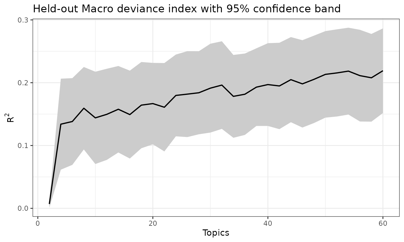
The band quantifies the uncertainty in the average held-out fit across evaluation documents, conditional on the trained models. The summary table also reports the Micro index, which weights each document by its baseline discrepancy, and the Micro-Macro gap with its standard error; a gap far from zero indicates that fit quality varies systematically with document weight.
The curve flattens quickly, and reading a single best K off it would
ignore the sampling noise. optop_gain_table() makes the
choice formal: for each adjacent pair of topic counts it computes the
paired per-document improvement in the held-out index, its one-sided
upper confidence bound, and a test of the hypothesis that the
improvement is zero.
gt <- optop_gain_table(ho, metric = "deviance", epsilon = 0.01)
show_upto <- if (identical(ho_res$selection_status, "selected")) {
  selected_gain <- match(ho_res$k_hat, ho_res$gains$K)
  min(nrow(ho_res$gains), selected_gain + 2L)
} else {
  min(nrow(ho_res$gains), 6L)
}
knitr::kable(
  ho_res$gains[seq_len(show_upto), ],
  digits = 4,
  caption = sprintf("Paired adjacent gains in the held-out deviance index (first %d of %d rows)",
                    show_upto, nrow(ho_res$gains))
)| K | succ_K | n | gain | sd | upper | z | pval |
|---|---|---|---|---|---|---|---|
| 2 | 4 | 15 | 0.1271 | 0.1442 | 0.1883 | 3.4136 | 0.0003 |
| 4 | 6 | 15 | 0.0042 | 0.0299 | 0.0169 | 0.5511 | 0.2908 |
| 6 | 8 | 15 | 0.0211 | 0.0271 | 0.0327 | 3.0169 | 0.0013 |
| 8 | 10 | 15 | -0.0153 | 0.0374 | 0.0006 | -1.5861 | 0.9436 |
| 10 | 12 | 15 | 0.0056 | 0.0404 | 0.0228 | 0.5405 | 0.2944 |
| 12 | 14 | 15 | 0.0081 | 0.0302 | 0.0209 | 1.0364 | 0.1500 |
Each row compares K with its successor on the same evaluation
documents: gain is the average paired improvement,
upper its one-sided 95% upper confidence bound, and
pval tests whether the improvement exceeds zero. The
selection rule fixes a tolerance epsilon, the improvement judged too
small to matter, before looking at the results, and picks the smallest K
at which even the optimistic end of the next gain falls below it.
With epsilon = 0.01, the rule selects K = 8: the step out of 8 is the first whose upper bound falls below the tolerance, so no gain of practical size is compatible with the data at that step.
A scalar index says how much error remains, not where. The moment tests of Lewis and Grossetti (2026) complement it by grouping the vocabulary into labeled word sets built from the training sample, the instruments, and testing whether the model consistently over- or under-predicts any group on the evaluation documents. Here we stratify the vocabulary by training frequency and compare each stratum against the highest-frequency reference:
k_diagnostic <- gt$k_hat
if (is.na(k_diagnostic)) {
  dev <- ho$summary[ho$summary$metric == "deviance", ]
  k_diagnostic <- dev$K[which.max(dev$macro)]
}
m_star <- VEM_train[[which(seq(2, 60, by = 2) == k_diagnostic)]]
mt <- optop_moment_test(list(m_star), dfm_eval, dfm_train,
                        type = "strata", bins = 5)
knitr::kable(
  ho_res$moment_marginal,
  digits = c(0, 5, 5, 2, 4, 4),
  format.args = list(scientific = FALSE),
  caption = sprintf("Marginal frequency-strata moments at K = %d",
                    ho_res$k_diagnostic)
)| stratum | estimate | se | t | pval | pval_adj |
|---|---|---|---|---|---|
| freq_1_vs_5 | 0.00013 | 0.00002 | 5.26 | 0.0000 | 0.0000 |
| freq_2_vs_5 | 0.00003 | 0.00002 | 1.25 | 0.2124 | 0.2124 |
| freq_3_vs_5 | 0.00002 | 0.00002 | 1.00 | 0.3193 | 0.3193 |
| freq_4_vs_5 | 0.00002 | 0.00002 | 0.71 | 0.4787 | 0.4787 |
The joint Wald statistic at K = 8 is 267.26 on 4 degrees of freedom
(p < 1e-15); with 15 evaluation documents the chi-square reference is
an asymptotic yardstick, and the marginal t statistics are the more
stable guide. In the marginal table, estimate is an effect
size in probability-mass units: a positive value means the held-out
documents place more mass on that frequency stratum than the model
predicts, relative to the reference stratum, and a negative value the
reverse. Here the largest imbalance sits in the lowest-frequency
stratum, with an estimate of about 0.00013 in probability mass:
statistically unambiguous, yet small in practical terms. Reading the
estimates alongside the p-values in this way separates detectable
imbalances from practically negligible ones.
Three caveats close the discussion of the single split. First, all confidence statements are conditional on the trained models: they quantify variability across evaluation documents, not across refits of the grid. Second, selecting K on this same evaluation sample, or choosing a diagnostic K from it when the adequacy rule does not select one, makes the reported diagnostic descriptive and subject to post-selection bias. A study that needs both a data-driven choice and clean inference at that choice should select on one evaluation sample and report on another, or rotate the roles of the splits. Third, a moment test that fails to reject does not certify the model class; it states that no systematic residual imbalance is detectable along the chosen instruments at the available sample size. The first two caveats have a standard remedy, and the package implements it.
V-Fold Cross-Fitting
optop_crossfit() rotates the roles of the splits
systematically (Appendix B of the paper): the documents are dealt into
V length-balanced folds, the model grid
is refit on each fold’s complement by a fitting function you supply, and
each fold is scored held-out through exactly the machinery of the
previous subsections. Every document is thus evaluated once, by models
that never saw it, and no single arbitrary split decides the
analysis.
fit_vem <- function(dtm_train, k) {
  topicmodels::LDA(quanteda::convert(quanteda::as.dfm(as.matrix(dtm_train)),
                                     to = "topicmodels"),
                   k = k, method = "VEM", control = list(seed = 3000 + k))
}
cf <- optop_crossfit(dtm_counts, K = c(10, 20, 30, 40, 50),
                     fit_fun = fit_vem, V = 5,
                     metrics = "deviance", seed = 20260722)
plot(cf)
Two things change relative to a single split. Point estimates pool the out-of-fold scores of the whole corpus, so no document is spent on training only. And the standard errors are fold-replicate estimates: the V per-fold values of each quantity are treated as exchangeable replicates, so the reported uncertainty includes the fold-to-fold variation induced by refitting, precisely what the first caveat said a single split cannot see. The price is that only V replicates feed each standard error, which is why small corpora get a warning about noisy fold means.
On the inaugural corpus (60 speeches, V = 5, coarse grid K = 10, 20, 30, 40, 50), the cross-fitted adequacy rule at epsilon = 0.01 selects K = 30: the first step out of that grid point has a fold-replicate upper bound below the tolerance. At K = 30 the pooled Macro deviance index is 0.2007 with a fold-replicate standard error of 0.0167. The single-split analysis above worked on a finer grid, so the two analyses answer slightly different questions; what matters is that the cross-fitted result is reproducible under the fold seed and spends every document on both sides of the fence exactly once.
A Simulation with Known Truth
In empirical corpora the true number of topics is unknown. Following
the paper, we therefore validate the procedure through a simulation
study in which the ground truth is known: one corpus is simulated from
the LDA generative process itself, with 100 documents over 1500 words
drawn from 10 topics, using the package’s own
sim_dfm() generator, and a grid of models is re-estimated
around the truth.
rdirichlet <- function(n, alpha) {
  g <- matrix(rgamma(n * length(alpha), shape = alpha, rate = 1),
              nrow = n, byrow = TRUE)
  g / rowSums(g)
}

set.seed(20260703)
true_K <- 10L
Theta_true <- rdirichlet(100L, rep(0.3, true_K))    # documents x topics
Beta_true <- rdirichlet(true_K, rep(0.05, 1500L))   # topics x words
doc_len <- sample(500:1500, 100L, replace = TRUE)

sim_corpus <- sim_dfm(DTW = Theta_true, TWW = Beta_true,
                      doc_length = doc_len, seed = 42)

sim_models <- parallel::mclapply(
  seq(2, 20, by = 2),
  function(k) topicmodels::LDA(sim_corpus, k = k,
                               control = list(seed = 2000 + k)),
  mc.cores = ncores
)

sim_chi <- optop_select(sim_models,
                        quanteda::dfm_weight(sim_corpus, scheme = "prop"),
                        q = 0.95, alpha = alpha, verbose = TRUE)
ggplot(sim_chi, aes(x = topic, y = OpTop)) +
  geom_line(linewidth = 0.8, color = "royalblue") +
  geom_vline(xintercept = meta$true_K, color = "red", linetype = 1) +
  geom_vline(xintercept = sim_picks$sequential, linetype = 2) +
  geom_vline(xintercept = sim_picks$min, linetype = 3) +
  labs(x = "Topics", y = expression(OpTop[J]^{K}),
       title = "Simulated corpus with ground truth K = 10 (solid red)",
       subtitle = sprintf("sequential pick: K = %d (dashed) | global minimum: K = %d (dotted)",
                          sim_picks$sequential, sim_picks$min)) +
  theme_bw()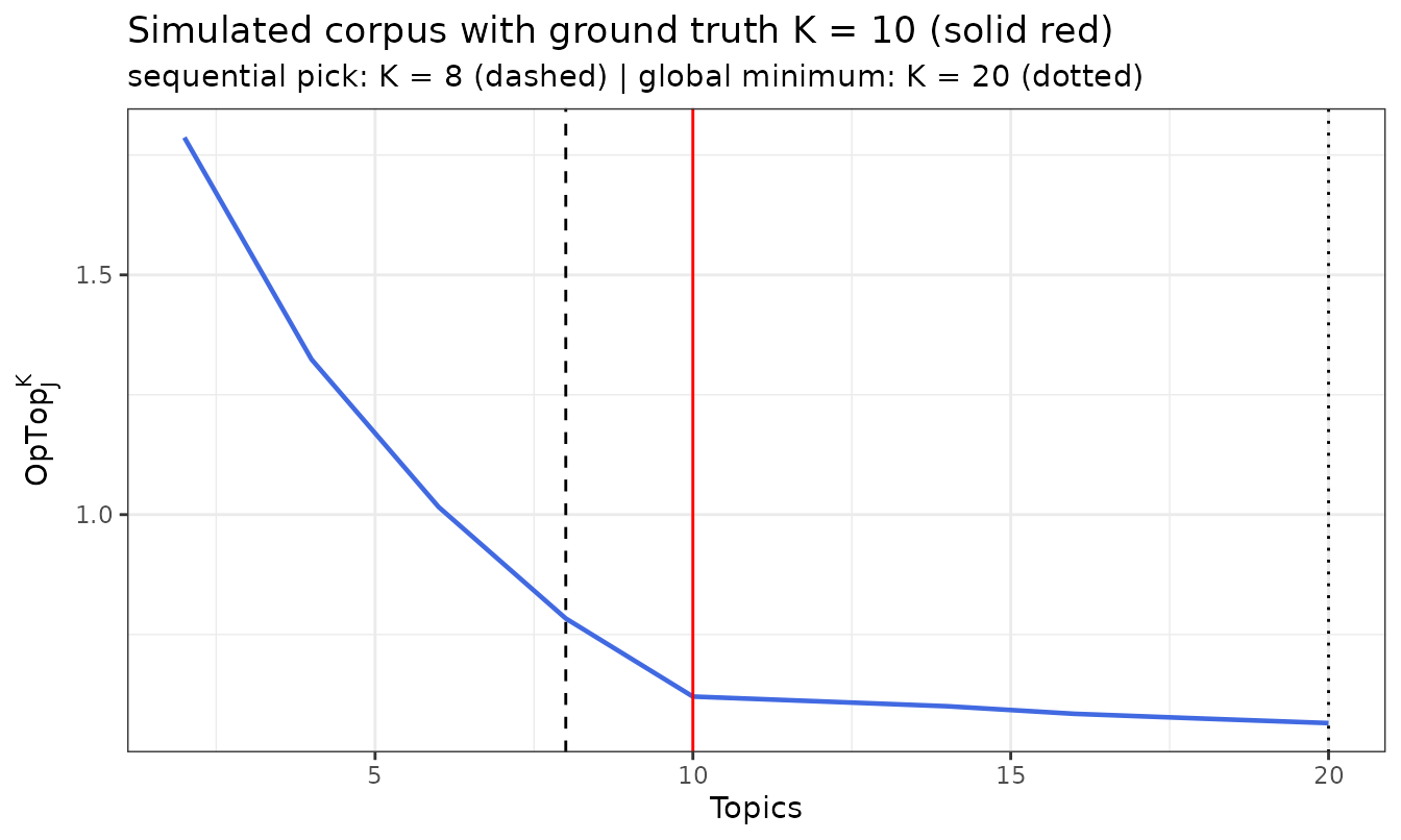
sim_idx <- melt(sim_idx_tab,
                id.vars = "K",
                measure.vars = c("R2_SE", "R2_chisq", "R2_dev"),
                variable.name = "metric", value.name = "R2")

ggplot(sim_idx, aes(x = K, y = R2, color = metric)) +
  geom_line(linewidth = 0.7) +
  geom_vline(xintercept = meta$true_K, color = "red", linetype = 1) +
  labs(x = "Topics", y = expression(R^2),
       title = "Discrepancy indices on the simulated corpus") +
  theme_bw()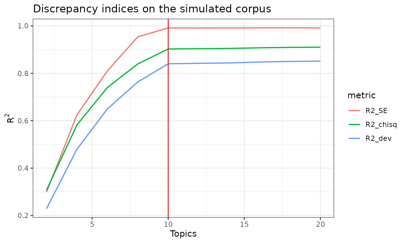
The statistic bends in the neighborhood of the true K and the indices stop improving there, the same qualitative behavior reported in the paper’s simulation study (its Figure 7). As the paper acknowledges, the identified optimum is not always exactly K_{sim} but is typically adjacent or in close proximity to it: here the sequential rule stops at K = 8 with the truth at 10, while the global minimum moves toward the grid boundary as the curve continues to decrease past the bend. Note that this is the uncalibrated sequential rule performing well. On this corpus the post-truth plateau of the standardized statistic lies below 1, so the implicit reduced-chi-square threshold of the saturated p-values falls close to the actual null level, which is the favorable case discussed in the calibration section. The tools should be read as locating the region of adequate K, with the discrepancy indices quantifying the incremental explanatory power of each candidate.
Other Engines and Bare Matrices
Everything above ran on topicmodels fits, but nothing in
the method is tied to an estimator. Fits from topicmodels
(VEM and Gibbs, and CTM), seededlda, and NLPstudio are
recognized directly: pass them to any OpTop function and the adapter
layer extracts the two weight matrices behind the scenes. Two more doors
cover everything else.
text2vec WarpLDA. The WarpLDA sampler splits its
output in two: fit_transform() returns the
document-topic matrix while the model object retains only the topic-word
distribution. optop_warplda() bundles the two halves into
one object that behaves like any supported fit, held-out fold-in
included:
lda <- text2vec::LDA$new(n_topics = k_star)
theta <- lda$fit_transform(dtm_counts, n_iter = 500, progressbar = FALSE)
fit <- optop_warplda(lda, theta)

warp_part <- optop_make_partition(list(fit), dtm_counts, c = 1)
warp_dev <- optop_index_deviance(fit, dtm_counts, warp_part, baseline,
                                 macro = TRUE)
Run on the inaugural corpus at K = 34, the WarpLDA fit reaches a micro deviance index of 0.3938 against 0.8804 for the VEM fit of the same size: the indices compare engines on one scale, which is precisely their purpose.
Any other engine. If your estimator only hands you
matrices, wrap them yourself: optop_model() validates the
full contract (named documents and terms, nonnegative weights, unit row
sums) and returns an object every in-sample tool accepts.
rdirich <- function(n, k) {
  g <- matrix(stats::rgamma(n * k, shape = 1), n, k)
  g / rowSums(g)
}
set.seed(11)
theta_toy <- rdirich(5, 2)
rownames(theta_toy) <- sprintf("doc%d", 1:5)
phi_toy <- rdirich(2, 8)
colnames(phi_toy) <- sprintf("w%02d", 1:8)

m_toy <- optop_model(theta_toy, phi_toy)
m_toy
#> <optop_theta_phi>: a topic model for OpTop
#> K = 2 topics, 5 documents, 8 terms
#> theta: 5 x 2, phi: 2 x 8; rows sum to 1
One limitation is structural: a bare matrix pair carries no fitted
engine, so new documents cannot be folded in and the held-out tools
refuse an optop_model() with a pointed message. Held-out
evaluation always wants the engine’s own object.
A closing practical note: OpTop aligns by term name, never by
position. If the document-term matrix and the models drift apart (a
trimmed feature, a reordered vocabulary), the index functions stop and
point at optop_align_dtm_to_models(), which subsets and
reorders the counts to the grid’s common vocabulary; recompute the
partition and the baseline on the aligned matrix afterwards.
A Note On Computational Efficiency
Both computational stages of optop_select() are
implemented in compiled code and, as of v0.12.0, run in parallel. The
same design extends to the goodness-of-fit tools presented above, whose
partition and index computations are evaluated by a fused compiled
engine. This section describes the implementations and reports a
simulation study of their speed, thread scaling, and memory use.
The statistic. For each model, the fitted word probabilities of a block of 256 documents are obtained with a single BLAS matrix product, since the per-document algebra of Equation (3) reduces to one row of the matrix product \theta^K \phi^K. The remaining per-document work (a descending sort, a cumulative sum, and a scalar Pearson reduction), which profiling identified as the dominant cost once the algebra had been reduced to a matrix product, is parallelized over the documents of each block with OpenMP.
The bootstrap. Calibration is the most expensive
stage: it draws B null replicates of
the statistic per model, each requiring one multinomial draw per
document. Since v0.12.0 the draws are generated in compiled code and
fused with the Pearson reduction, so that no intermediate count matrices
are materialized, and the document loop is parallelized. The sampler is
chosen per document from the data alone: when the envelope holds more
bins than the document holds tokens, the common regime on large
vocabularies, the tokens are drawn directly through an alias table at
O(N_j) per replicate and the untouched
bins contribute a closed-form Pearson term; otherwise the
conditional-binomial method is used. Each document draws from a private
random-number stream seeded deterministically from the pair
(seed, document index), and all reductions are performed in
a fixed order. Two properties follow: the output is bit-identical for
every value of n_threads, which therefore affects wall time
only, and the calibrated p-values are reproducible under
seed.
The study below evaluates VEM grids of ten models (five on the
largest corpus) on four synthetic corpus scales, from J = 200 documents
with W = 2,000 features up to J = 10,000 documents with W = 20,000
features, timing the statistic pass, the bootstrap-calibrated pass (B =
200), and the goodness-of-fit evaluation for one, two, and four threads,
with the corresponding pure-R implementations as baselines. The sweep
ends at four threads because that is the host’s logical core count;
thread settings beyond the physical cores only measure oversubscription,
so the benchmark driver caps the sweep at the core count and extends it
automatically on machines with more cores. Peak memory is the maximum
resident set size reported by the operating system for a fresh R process
per configuration. The study is reproducible via
data-raw/benchmark-efficiency.R; timings are
machine-dependent (recorded here: Intel(R) Xeon(R) Processor @ 2.10GHz,
4 logical cores, R version 4.3.3 (2024-02-29)).
| scale | J | W | R bootstrap (0.11.0) | C++ bootstrap, 1 thread | C++ bootstrap, 2 threads | C++ bootstrap, 4 threads |
|---|---|---|---|---|---|---|
| small | 200 | 2000 | 33.5 | 18.1 | 9.2 | 4.7 |
| medium-1 | 500 | 5000 | 165.9 | 31.3 | 16.0 | 8.7 |
| medium-2 | 1000 | 10000 | 579.2 | 67.0 | 36.1 | 20.5 |
| large | 10000 | 20000 | 6407.4 | 421.0 | 232.8 | 141.9 |
| scale | J | W | 1 thread | 2 threads | 4 threads |
|---|---|---|---|---|---|
| small | 200 | 2000 | 0.37 | 0.26 | 0.18 |
| medium-1 | 500 | 5000 | 2.29 | 1.34 | 0.81 |
| medium-2 | 1000 | 10000 | 9.36 | 5.19 | 3.20 |
| large | 10000 | 20000 | 109.92 | 61.66 | 37.16 |
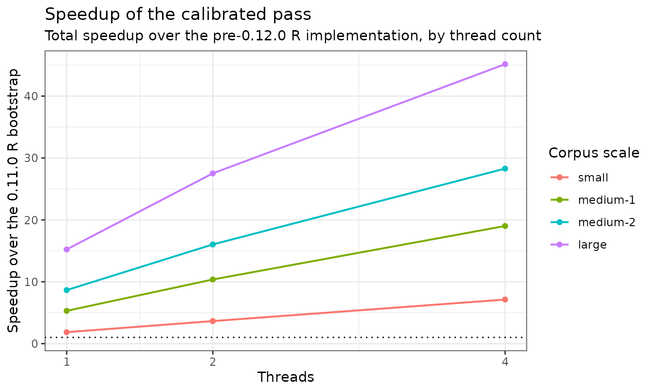
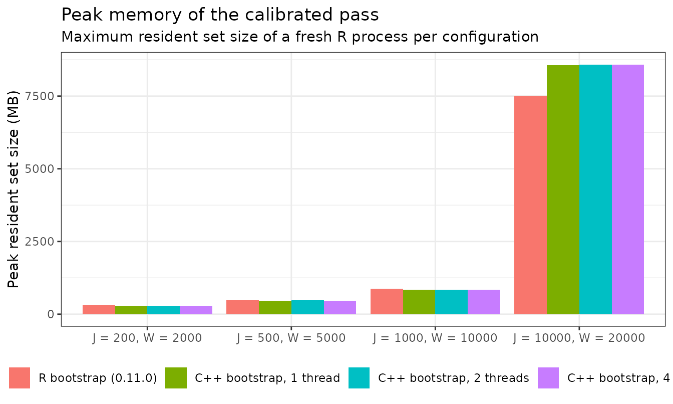
Three regularities hold across the scales. First, the compiled
bootstrap is 1.9–15.2× faster than the R implementation before any
threading, and the gain grows with the vocabulary: the alias-table path
costs O(N_j) per replicate where the
bin-wise method costs O(k_j), and wide
corpora have k_j \gg N_j. Second, the
parallel document loop scales almost linearly in the number of physical
cores: the best configuration on the largest corpus (4 threads) runs the
calibrated pass 45.2× faster than the 0.11.0 baseline, falling from
106.8 minutes to 142 seconds. The statistic pass shares the
document-level parallelism and gains 3.0× at its best thread setting on
the same corpus; its speedup is sub-linear because the BLAS product
remains serial. Third, peak memory is governed by the objects the
evaluation must hold, namely the fitted models and, on the largest
corpus, the exported envelope bins, rather than by the sampling itself:
the two implementations stay within roughly 15% of one another in either
direction, and the per-thread state amounts to one result slot per
document, so peak memory does not grow with n_threads.
The discrepancy indices. The goodness-of-fit tools
presented above follow the same design. The harmonized partition of
optop_make_partition() keeps the running minimum across the
model grid one vocabulary block at a time in compiled code, so the full
J \times W minimum matrix is never
materialized, and the three discrepancy indices are evaluated by a fused
engine that computes all requested metrics, for the model and for the
no-topics baseline side, in a single traversal of each document block.
The evaluation consumes the sparse counts directly, forms the baseline
on the fly, and parallelizes over documents under the contract stated
above: results are bit-identical for every value of
n_threads, exposed on the index functions and on
optop_make_partition(). The table reports the wall time of
the full evaluation, the partition followed by a three-metric
document-level optop_index_table() over the grid, with the
vectorized R implementation that preceded the engine as baseline. The
rare-word threshold is set so that the harmonized support remains
non-trivial at every scale of these synthetic corpora; the computational
cost of the evaluation does not depend on that choice.
| scale | J | W | R base (pre-engine) |
C++ base 1 thread |
C++ base 2 threads |
C++ base 4 threads |
|---|---|---|---|---|---|---|
| small | 200 | 2000 | 1.0 | 0.2 | 0.2 | 0.1 |
| medium-1 | 500 | 5000 | 6.4 | 0.9 | 0.7 | 0.7 |
| medium-2 | 1000 | 10000 | 33.1 | 3.7 | 3.2 | 3.0 |
| large | 10000 | 20000 | 331.3 | 39.8 | 35.4 | 32.9 |
On the largest corpus the evaluation falls from 5.5 minutes to 32.9 seconds at 4 threads, a 10.1-fold reduction, and peak memory falls from 9.0 GB to 3.2 GB, since neither the minimum matrix nor the dense count and baseline blocks are formed.
On toolchains without OpenMP support (notably the default macOS
compiler) the parallel loops run single-threaded; the thread-independent
speedup of the compiled bootstrap and of the index engine is retained,
while the scaling with n_threads is not. The internal
helper OpTop:::optop_openmp_available() reports whether the
installed build supports OpenMP.
Very large corpora
As of version 0.15.0 the package evaluates corpora of tens of
millions of documents with bounded memory, exactly. Three design
elements carry the scaling. First, the corpus crosses the compiled
boundary as zero-copy views of the sparse matrix slots, so no copy of
the corpus is ever made and its shape is unconstrained. Second, the
harmonized partition stores the complement of the rare set, the
per-document non-rare word lists, whose total size is bounded by the
token count divided by c; the construction evaluates only
the candidate cells whose baseline probability clears the document
threshold, so its cost scales with the token count rather than with the
documents-by-features product, and no dense documents-by-features object
of any kind is materialized. Third, corpora larger than a single sparse
matrix can hold (the container caps at 2^31 - 1 nonzero entries) are
supplied as document shards through optop_corpus(), which
every entry point accepts; shards are streamed one at a time,
per-document results are bit-identical to an unsharded run, and the
calibration bootstrap keys each document’s random stream by its global
index. Model grids too large for memory are supplied as loader
functions, materialized one model at a time. The package website article
OpTop
at very large scale is the operations manual for this regime:
sharding, loaders, the cache budget, thread and BLAS configuration, and
memory planning with the reference timings of the scale benchmark.
Notes
- The pre-0.9.8 stability helpers and the
selection = "legacy"rule were removed in 0.16.0 after a long deprecation; the discrepancy indices shown here are their replacement. - The chi-square reference for Test 1 is asymptotic rather than exact;
the calibrated p-values presented above
(
calibrate = "bootstrap"orcalibrate = "moment") address this, and?optop_selectdocuments the underlying statistical reasoning.
References
Haldane, J. B. S. (1937). The exact value of the moments of the distribution of chi-square. Biometrika, 29, 133–143.
Lewis, C. M. and Grossetti, F. (2022). A statistical approach for optimal topic model identification. Journal of Machine Learning Research, 23(58), 1–20. https://jmlr.org/papers/v23/19-297.html
Lewis, C. M. and Grossetti, F. (2026). Goodness-of-fit indices and diagnostics for topic models. Working paper.